Bayes’ theorem is one of the most useful applications in statistics. But sometimes it is not always easy to recognize when and how to apply it. I was doing some statistics problems with my Insight cohort when applying conditional probability in one, simpler problem helped me connect it with a slightly harder, baseball-related problem.
In this post, I’ll go over a couple of applications of Bayes!
# Load packages for coding examples
import pandas as pd
import numpy as np
from scipy.stats import binom
import matplotlib.pyplot as plt
import seaborn as sns
Bertrand’s box paradox
The first problem came from my old textbook. The problem is famous, but I’m apparently not with the in-crowd because I was not aware of it. It’s called Bertrand’s box paradox.
A box contains three drawers: one containing two gold coins, one containing two silver coins, and one containing one gold and one silver coin. A drawer is chosen at random, and a coin is randomly selected from that drawer. If the selected coin turns out to be gold, what is the probability that the chosen drawer is the one with two gold coins?
The drawers can be referred to like this:
Box A: G,G
Box B: S,S
Box C: G,S
I’m going to show a few different approaches for the problems. One reason for this is that you can see how the answer can be confirmed. (Again, since this problem is well-known, you might find other explanations helpful, including on the problem’s entry in Wikipedia.) But another reason is to point out some flaws in these other approaches, compared to how application of Bayes’ theorem can be robust.
“Reasoning” approach
One way to approach this is to “reason” your way through the problem. Let’s say that each of the boxes has two drawers. The problem can be re-framed as, “If you randomly choose a box, and then find a gold coin in one of the drawers, what is the probability that the other will be a gold coin?” You can eliminate box B (S,S). Many believe that since the coin must come from either box A or box C, there is a 50% chance that the gold coin must come from box A. However, this is not the correct answer (and also why it’s referred to as a paradox). The right approach would be to consider that the selected gold coin is one of the following three gold coins:
- gold coin 1 from box A
- gold coin 2 from box A
- gold coin 3 from box C
Therefore, it’s a 2/3 probability that it comes from box A. While this approach may help you get an answer quickly, it relies on making the proper assumptions. But the correct suppositions are not always obvious without regular experience doing problems like this. Accordingly, the “reasoning” method must be applied with caution.
Experimental simulation approach
A second approach can be taking repeated trials through code and seeing where the answer converges. This would be an application of the law of large numbers. Here is some code where I first randomly choose one of the three boxes and then randomly choose one of the two coins in that box. (For box C, which contains a gold and silver coin, I assign drawer 1 as the gold coin and than randomly choose between drawers 1 and 2.)
# Code to run a lot of trials

from collections import Counter
import random

boxes = ["A", "B", "C"]
coin_side = [1, 2]  # Assume gold is on drawer 1 of Box C

box_count = Counter()
box_count_wgold = Counter()
prob_A_list = list()

for trial in range(10**5):
    # Randomly pick a box
    box = random.sample(boxes, 1)[0]
    box_count[box] += 1

    # Randomly pick coin after picking a box
    if box == "A":
        box_count_wgold[box] += 1  # we know it will always be gold for box A

    elif box == "C":
        side = random.sample(coin_side, 1)[0]  # assume gold is on drawer 1 of Box B
        if side == 1:
            box_count_wgold[box] += 1

    # Ignore box B (silver, silver box)

    # This is calculating the probability after each trial, starting at trial 10
    if trial > 10:
        prob_A_list.append(box_count_wgold["A"] / (box_count_wgold["A"] + box_count_wgold["C"]))
sns.set_context('talk')
f, ax1 = plt.subplots(figsize=(12,6))
ax1.plot(prob_A_list, color='gray')
ax1.axhline(0.6667, color='r', linestyle='dashed', linewidth=1)
ax1.set_xlabel('trial')
ax1.set_ylabel('probability')
ax1.set_title('Probability that gold is from box A \n(updating after each trial)')
ax1.text(35000, 0.675, 'red dashed line is at 0.667', color='r', fontsize=12);
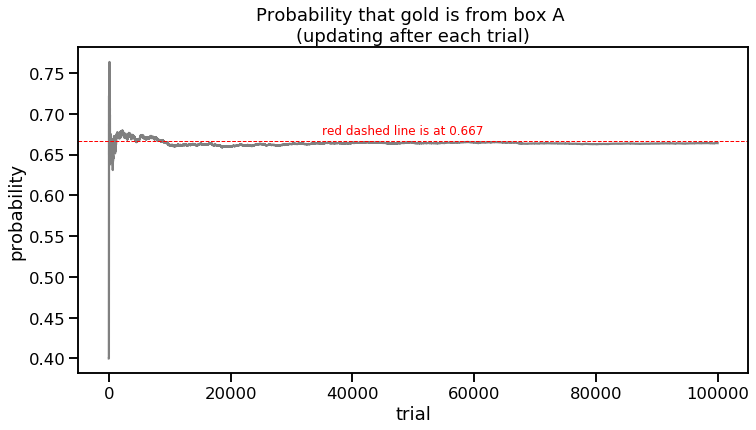
print("Probability after 100,000 trials: {0:0.4f}".format((box_count_wgold["A"] / (box_count_wgold["A"] + box_count_wgold["C"]))))
Probability after 100,000 trials: 0.6641
One advantage of the simulation approach is that not many assumptions have to be made. One can simply use code to carry out the parameters of the problem repeatedly. However, as you can see, even after 100,000 trials, we don’t get 2/3 exactly. Bayes to the rescue!
Bayesian approach
Let’s remind ourselves how Bayes’ theorem uses conditional probability.
| $\text{P}(A | B) = \frac{\text{P}(B | A)\text{P}(A)}{\text{P}(B)}$ |
Huh? Let’s translate the terms into words.
| $\text{P}(A | B)$ = The probability of event A occurring given that B is true. The left side of the equation is what we are trying to find. |
The entire right side of the equation is information that we are given (although we have to make sure we put in the right numbers).
$\text{P}(B|A)$ = The probability of event B occurring given that A is true. This is not equivalent to the left side of the equation.
$\text{P}(A)$ = The probability of event A occurring, regardless of conditions.
$\text{P}(B)$ = The probability of event B occurring, regardless of conditions.
Another way of stating the problem is asking “What is the probability that the box chosen is A, given that you have also selected a gold coin?” Substituting the words in to Bayes’ theorem would give us something like this:
| $\text{P}(\text{box A} | \text{gold coin}) = \frac{\text{P}(\text{gold coin} | \text{box A})\text{P}(\text{box A})}{\text{P}(\text{gold coin})}$ |
The entire right side of the equation is information that we are given. The parameters in the numerator are the easiest for which we can plug in numbers.
We know that there is 100% probability of picking a gold coin if we choose box A.
$\text{P}(\text{gold coin} | \text{box A})$ = 1
We are choosing box A randomly out of the 3 boxes.
$\text{P}(\text{box A})$ = 1/3
The denominator ($\text{P}(\text{gold coin}$) might require a closer look. The probability of choosing a gold coin, independent of any other condition, is the sum of the probability of choosing a gold coin in the three boxes.
| $\text{P}(\text{gold coin})$ = $\text{P}(\text{gold coin} | \text{box A})$ + $\text{P}(\text{gold coin} | \text{box B})$ + $\text{P}(\text{gold coin} | \text{box C})$ |
$\text{P}(\text{gold coin})$ = $1 \times \frac{1}{3} + 0 \times \frac{1}{3} + \frac{1}{2} \times \frac{1}{3}$
$\text{P}(\text{gold coin})$ = $\frac{1}{2}$
Therefore,
| $\text{P}(\text{box A} | \text{gold coin}) = \frac{1 \times \frac{1}{3}}{\frac{1}{2}} = \frac{2}{3} $ |
Awesome. This is how we apply Bayesian statistics in this problem. Let’s level up and try a problem that is a little more complicated, using a baseball scenario as an example.
Bayes-ball
Let’s imagine that there are only two types of hitters in MLB, those with a true talent 10% hit rate and those with a true talent 25% hit rate. We also know that 60% of MLB hitters are in the 10% hit rate group and the remaining 40% are in the 25% hit rate group. Suppose we have observed a hitter, Bobby Aguila, over 100 plate appearances and he has hit at an 18% rate. What is the probability that Aguila has a true talent level of 10% hit rate?
Bayes’ theorem can be applied here but it may take a little more digging to see it. Let’s create some notations before we get started.
T10 = true talent 10% hit group
T25 = true talent 25% hit group
18H = 18 hits in 100 at-bats
The original question could be phrased as “What is the probability that Aguila has a true talent level of 10% hit rate, given that he has 18 hits in 100 at-bats?”
In Bayes’ theorem, we can therefore structure our equation like this:
| $\text{P}(\text{T10} | \text{18H}) = \frac{\text{P}(\text{18H} | \text{T10})\text{P}(\text{T10})}{\text{P}(\text{18H})}$ |
Connecting with Bertrand’s box paradox
The easiest parameters to plug in is the probability that the hitter, in the absence of any condition (without knowing anything else), is from the T10 group. We were given that explicitly in the problem:
$\text{P}(\text{T10})$ = 0.60
Note that this is analogous to $\text{P}(\text{box A})$ in Bertrand’s box problem. In that problem, we knew the value implicitly ($\frac{1}{3}$) since the drawer was chosen at random.
The other parameters of the baseball question are less obvious to determine, but we can get some clues after translating back to words. Let’s start with $\text{P}(\text{18H})$. This is equivalent to ${\text{P}(\text{gold coin})}$ in Bertrand’s box paradox. In the box problem, we broke this down by summing up the probabilities for a gold coin for each drawer. Here, we would sum up the probabilities of a hitter getting 18 hits in 100 at-bats if he is in the T10 group and in the T25 group.
| ${\text{P}(\text{18H})}$ = $\text{P}(\text{18H} | \text{T10})$ + $\text{P}(\text{18H} | \text{T25})$ |
| $\text{P}(\text{18H} | \text{T10})$ is asking “What is the probability of getting 18 hits in 100 at-bats, given that they have a true talent level of 10% hit rate?” $\text{P}(\text{18H} | \text{T25})$ is basically the same question but for the T25 group. Here is where we need to recognize that this is an application of the binomial distribution. Let’s digress briefly. |
Application of the binomial distribution
This problem fits the binomial assumptions:
- Two outcomes: For each plate appearance, we care that he is getting a hit (1) or no hit (0).
- Constant p: The probability p getting a success has the same value, for each trial. This would be 0.10 for the group that has a 10% hit rate true talent level and 0.25 for the T25 group.
- Independence: This is the one assumption that may be potentially violated since a hitter’s confidence may fluctuate based on recent performance. However, in this situation I think it is okay to assume at-bats are largely independent of each other.
The probability mass function is: $\text{P}(X = k) = \binom n k p^k(1-p)^{n-k}$
where: $\binom n k = \frac{n!}{(n-k)!k!}$ (the binomial coefficient).
In this problem, k = 18 and n = 100. And as mentioned above, the T10 group has p = 0.10 while T25 has p of 0.25. We can start plugging values in. However, this visual may also help see what is going on.
from scipy.stats import binom

# T10 group
n, p = 100, 0.1
fig, ax = plt.subplots(1, 1, figsize=(12, 6))
rv = binom(n, p)
x = np.arange(0, 45)
ax.vlines(x, 0, rv.pmf(x), colors="k", linestyles="-", lw=2, label="T10")

# T25 group
n25, p25 = 100, 0.25
rv25 = binom(n25, p25)
x25 = np.arange(0, 45)
ax.vlines(x25 + 0.2, 0, rv25.pmf(x25), colors="r", linestyles="-", lw=2, label="T25")

# Formatting
ax.set_ylabel("probability")
ax.set_xlabel("number of hits")
ax.set_title("Probability distribution after 100 plate appearances")

# Box around 18 hits
ax.text(16.5, 0.04, '18 hits', color='b', fontsize=12);
ax.vlines(17.6, -0.0025, 0.035, colors="blue", linestyles="-", lw=1)
ax.vlines(18.6, -0.0025, 0.035, colors="blue", linestyles="-", lw=1)
ax.hlines(0.035, 17.6, 18.6, colors="blue", linestyles="-", lw=1)
ax.hlines(-0.0025, 17.6, 18.6, colors="blue", linestyles="-", lw=1)
ax.legend();
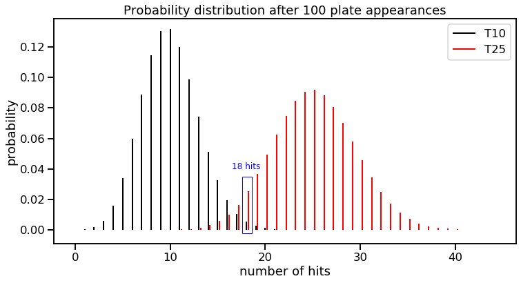
We can see that each true talent level group has its own probability distribution for different hits a hitter would get in 100 at-bats. Not surprisingly, the number of hits containing the highest probability for the respective groups are its true talent hit rate for 100 at-bats. In other words, we see 10 hits as being most probable in the T10 group and 25 hits as most probable in the T25 group.
Another observation you might make is that the T10 group has a tighter variance than the T25 group. This is a property of the binomial distribution, where variance is equal to $np \times (1-p)$. You can see that proportions that are closer to 0 or closer to 1, will have less variance than a proportion closer to the middle. (The Bernoulli distribution, which is just one trial of a binomial distribution, shows a similar property, something I wrote about in a previous post.)
The height of the black and red lines at 18 hits should add up to 1, but weighted by what we know about the two groups of baseball hitters (our “priors”). If we were to use the graph above, the probability of getting 18 hits in 100 at-bats, given that they have a true talent level of 10% hit rate would be:
| $\text{P}(\text{T10} | \text{18H}) = \frac{\text{height of black line at 18 hits} \times 0.6}{\text{height of black line at 18 hits} \times 0.6 + \text{height of red line at 18 hits} \times 0.4}$ |
Putting it all together
Let’s return to the parameters of the Bayes’ theorem equation and start bringing the pieces together.
| ${\text{P}(\text{18H})}$ = $\text{P}(\text{18H} | \text{T10})$ + $\text{P}(\text{18H} | \text{T25})$ |
We can apply the probability mass function starting first with the T10 group. (Note that we can ignore calculation of the binomial coefficient since this will cancel out in the final equation. I’ll use the term $\propto$ to represent “in proportion to.” in the equations below.)
| $\text{P}(\text{18H} | \text{T10}) \propto (0.1^{18} \times 0.9^{82}) $ |
| $\text{P}(\text{18H} | \text{T25}) \propto (0.25^{18} \times 0.75^{82}) $ |
We now have everything we need to plug into our equation.
| $\text{P}(\text{T10} | \text{18H}) = \frac{\text{P}(\text{18H} | \text{T10})\text{P}(\text{T10})}{\text{P}(\text{18H})}$ |
| $\text{P}(\text{T10} | \text{18H}) = \frac{(0.1^{18} \times 0.9^{82}) \times 0.6}{(0.1^{18} \times 0.9^{82}) \times 0.6 + (0.25^{18} \times 0.75^{82}) \times 0.4} $ |
| After all that math, we have (drumroll) $\text{P}(\text{T10} | \text{18H}) = 0.243$. |
Therefore, there is 24.3% probability that Aguila has a true talent level of a 10% hit rate.
The baseball example is also the diachronic interpretation** of Bayes’ theorem, which is a fancy way of saying that the hypothesis can be updated with time (in this case, after 100 plate appearances).