Rethinking Bayes

A few weeks ago, I learned about the wonderful Statistical Rethinking lecture series and book by Richard McElreath. It’s made me think about some of the Bayesian statistics I’ve learned a little bit more (which is a nicer way of acknowledging I was more ignorant than I realized). For example, I had to think a bit about the difference between a prior distribution and a prior predictive distribution. Fortunately, someone had already asked this in a nice StackExchange post. I could have stopped after the first few sentences of the accepted answer: “Predictive here means predictive for observations. The prior distribution is a distribution for the parameters whereas the prior predictive distribution is a distribution for the observations.”

The answer went on to explain in more detail. However, this tends to be my reaction when looking only at equations. In this post, I’ll show differences in distributions for prior, prior predictive, likelihood, posterior, and posterior predictive with a concrete example. We’ll use McElreath’s globe tossing example from his first two lectures.

He tosses an inflatable globe to a student and when they catch it, he asks whether their right index finger is touching land or water. The objective is to determine what proportion of the globe is covered by water. Like the lecture, we’ll do nine tosses of the globe with a little bit of a lemon twist: I’ll simply focus on the first six tosses, divided up into two datasets of three tosses each.

import matplotlib.pyplot as plt
import numpy as np
import os
import pandas as pd
import scipy.stats as stats
import seaborn as sns

%load_ext nb_black

<IPython.core.display.Javascript object>

def plot_beta(a_val, b_val, label_val, style, color, ax):
    """
    Analytical analysis to compare with sampling from grid approximation.
    """
    # Expected value of parameter
    mu = a_val / (a_val + b_val)

    # Lower, upper bounds of interval
    lower, upper = stats.beta.ppf([0.025, 0.975], a_val, b_val)

    # Main plot
    x_val = np.arange(0, 1, 0.01)
    ax.plot(
        x_val,
        stats.beta.pdf(x_val, a_val, b_val),
        color=color,
        lw=1,
        linestyle=style,
        label=label_val,
    )

<IPython.core.display.Javascript object>

Prior

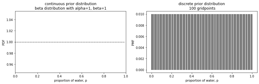
Before doing any tosses, we have not seen any data. Therefore, it’s reasonable to have a uniform prior for the proportion of water covering the globe. In other words, we are saying that all values between 0 and 1 are plausible. (Yes, I know this example is contrived.)

There are two ways we can represent the uniform prior distribution in this particular case. Use of the beta distribution is an example for the analytical case as shown on the left below. But using grid approximation will set us up for later scenarios where we use samples. That is what is shown on the right.

# Use a0 and b0 for our prior
# mu = 0.175
# total_ab = 100
a0, b0 = 1, 1
# print("a0, b0 values: ", a0, b0)

f, (ax1, ax2) = plt.subplots(1, 2, figsize=(12, 4))

# Analytical method, beta distribution (continuous)
plot_beta(a0, b0, "prior", "dashed", "black", ax1)
ax1.set_xlim([0, 1])
ax1.set_xlabel("proportion of water, p")
ax1.set_ylabel("PDF")
ax1.set_title(
    f"continuous prior distribution\nbeta distribution with alpha={a0}, beta={b0}"
)

# Grid approximation distribution (discrete)
n_gridpoints = 100
p_wat = np.linspace(0, 1, n_gridpoints)
prior0_vals = np.repeat(1 / n_gridpoints, n_gridpoints)  # specific to this question
ax2.vlines(p_wat, 0, prior0_vals)
ax2.set_ylabel("PMF")
ax2.set_xlabel("proportion of water, p")
ax2.set_title(f"discrete prior distribution\n {n_gridpoints} gridpoints")

plt.tight_layout()

<IPython.core.display.Javascript object>

The graphs look quite different because the left shows a continuous distribution while the right shows a discrete distribution. The point is that the total distribution in each case sums to 1 and that the values are flat across the possible values for the proportion of water. The key here is noting that the x-axis is a distribution of the parameter (in this case it is designated by p, but in other contexts it may be shown as $\theta$.)

Sampling the parameter values is a paradigm shift for me. The advantage of the grid approximation approach is that we can think of it as having a bag of numbers. In this scenario, I arbitrarily chose to have 100 gridpoints and each of those gridpoints is represented equally. It’s like having a marble for each in a bag. We pick one out, note the number on the marble, put it back, and repeat many times.

# Pulling a marble out of the bag 10,000 times
samples0 = np.random.choice(p_wat, p=prior0_vals, size=10 ** 4, replace=True)

# Take a look at the first 20 sampled parameter values
samples0[0:20]

array([0.4040404 , 0.64646465, 0.56565657, 0.83838384, 0.35353535,
       0.87878788, 0.02020202, 1.        , 0.78787879, 0.4040404 ,
       0.55555556, 0.02020202, 0.41414141, 0.32323232, 0.39393939,
       0.97979798, 0.05050505, 0.81818182, 0.31313131, 0.36363636])




<IPython.core.display.Javascript object>

Prior Predictive

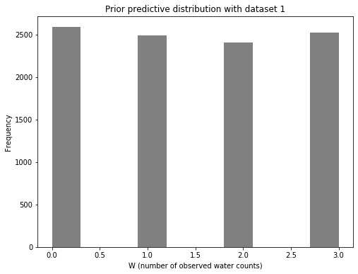
Now let’s look at the prior predictive distribution. This will be a distribution of count data: the number of water observations (designated by W). As a reminder, we are doing three tosses for each dataset, including this first one. Therefore, W can be 0, 1, 2, or 3.

# Use each sampled parameter for a binomial likelihood with n of 3
prior_pred = stats.binom.rvs(3, samples0, loc=0, size=10000, random_state=19)

# Take a look at the first 20 resulting W values
prior_pred[0:20]

array([0, 1, 2, 3, 1, 3, 0, 3, 1, 1, 2, 0, 1, 0, 0, 3, 0, 3, 1, 1])




<IPython.core.display.Javascript object>

f, ax1 = plt.subplots(1, 1, figsize=(8, 6))

ax1.hist(prior_pred, color="gray")
ax1.set_xlabel("W (number of observed water counts)")
ax1.set_ylabel("Frequency")
ax1.set_title("Prior predictive distribution with dataset 1")

Text(0.5, 1.0, 'Prior predictive distribution with dataset 1')

<IPython.core.display.Javascript object>

Given that the parameters we sampled from were uniformly distributed, we shouldn’t be surprised that the prior predictive distribution for the number of observed water counts is also uniform. Remember: this is only a check before we have seen any data.

Likelihood

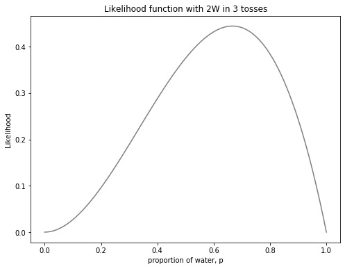
Now let us consider the data. In the scenario from the lecture, there were two waters and one land in the first three tosses. Before seeing the posterior, let’s plot the likelihood on its own. It was key to remember that the x-axis is also a plot of the parameter.

prob_data1 = stats.binom.pmf(k=2, n=3, p=p_wat)

f, ax1 = plt.subplots(1, 1, figsize=(8, 6))
ax1.plot(p_wat, prob_data1, color="gray")
ax1.set_xlabel("proportion of water, p")
ax1.set_ylabel("Likelihood")
ax1.set_title("Likelihood function with 2W in 3 tosses")

Text(0.5, 1.0, 'Likelihood function with 2W in 3 tosses')

<IPython.core.display.Javascript object>

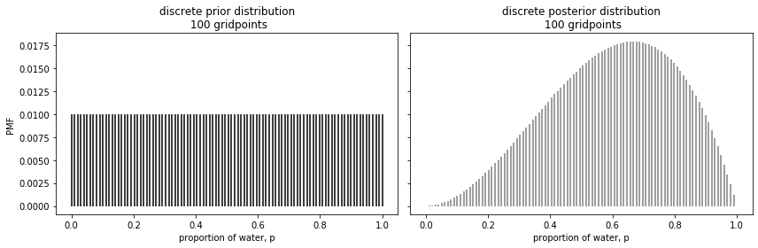
Posterior

Now let us use this new information to generate our posterior, generating a non-standardized and a standardized posterior in separate lines.

# Non-standardized posterior
posterior1_nonstd = prob_data1 * prior0_vals

# Standardized posterior
posterior1_std = posterior1_nonstd / np.sum(posterior1_nonstd)

<IPython.core.display.Javascript object>

f, (ax1, ax2) = plt.subplots(1, 2, figsize=(12, 4), sharey=True)

ax1.vlines(p_wat, 0, prior0_vals)
ax1.set_ylabel("PMF")
ax1.set_xlabel("proportion of water, p")
ax1.set_title(f"discrete prior distribution\n {n_gridpoints} gridpoints")


ax2.vlines(p_wat, 0, posterior1_std, color="gray")
# ax2.set_ylabel("PMF")
ax2.set_xlabel("proportion of water, p")
ax2.set_title(f"discrete posterior distribution\n {n_gridpoints} gridpoints")

plt.tight_layout()

<IPython.core.display.Javascript object>

Now let’s create the posterior predictive distribution.

# Pulling a marble out of the bag 10,000 times
samples1 = np.random.choice(p_wat, p=posterior1_std, size=10 ** 4, replace=True)

# Take a look at the first 20 sampled parameter values
samples1[0:20]

array([0.65656566, 0.2020202 , 0.53535354, 0.55555556, 0.85858586,
       0.53535354, 0.48484848, 0.61616162, 0.42424242, 0.50505051,
       0.57575758, 0.41414141, 0.55555556, 0.39393939, 0.83838384,
       0.62626263, 0.44444444, 0.56565657, 0.68686869, 0.92929293])




<IPython.core.display.Javascript object>

This is about having now parameter samples that are now differentially represented.

Posterior predictive

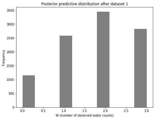
Now let’s look at the posterior predictive distribution. This will be a distribution of count data: the number of water observations (designated by W). As a reminder, we are doing three tosses for the next dataset. Therefore, W remains as 0, 1, 2, or 3.

# Use each sampled parameter for a binomial likelihood with n of 3
posterior_pred = stats.binom.rvs(3, samples1, loc=0, size=10000, random_state=19)

# Take a look at the first 20 resulting W values
posterior_pred[0:20]

array([3, 1, 2, 3, 3, 3, 2, 1, 3, 1, 2, 1, 2, 1, 3, 2, 0, 2, 2, 3])




<IPython.core.display.Javascript object>

f, ax1 = plt.subplots(1, 1, figsize=(8, 6))

ax1.hist(posterior_pred, color="gray")
ax1.set_xlabel("W (number of observed water counts)")
ax1.set_ylabel("Frequency")
ax1.set_title("Posterior predictive distribution after dataset 1")

Text(0.5, 1.0, 'Posterior predictive distribution after dataset 1')

<IPython.core.display.Javascript object>

Summary

In summary, I re-visited some Bayesian analysis concepts in the context of the Statistical Rethinking lessons. Specifically, I started with thinking about the differences between the “prior” and “prior predictive” terms and then extended that to “likelihood”, “posterior”, and “posterior predictive”. I think it should also be clear how the “posterior” and “posterior predictive” data here can serve as “prior” and “prior predictive” for a subsequent dataset if I chose to do another experiment.

Some keys for me in grasping these concepts was understanding what is being plotted on the x- and y-axes and also realizing how one can draw samples from simulated as an alternative to the analytical approach. These concepts are foundational to future lessons including hierarchical modeling applications.