
School and community features associated with low income student success
I originally shared this article more widely on Medium. I’ve seen taken that version down after I learned more about causal inference and Bayesian data analysis. I an opting to keep this version here, which showcases some skills even if some conclusions may be flawed. Learning is a journey and I don’t think it makes sense to hide our lessons along the way.
Summary
Low income students face academic challenges that affect long-term employment and upward social mobility. Fortunately, some schools provide environments for low income students to thrive. In this project, I investigated features of California (CA) public high schools and their communities that may affect low income student performance. I focused on a school’s percentage of low income students that are college eligible (SPLICE). College eligibility here is defined as meeting the subject and grade requirements for the University of California or California State University (CSU) systems. To obtain school-specific features, I acquired data from the CA public schools database and GreatSchools websites. This was supplemented with local economic characteristics from the census. Following data exploration and filtering, I built classification models to predict schools with exceptional SPLICE. Exceptional SPLICE is defined as a school achieving greater than one standard deviation above mean SPLICE across all CA high schools. A regularized logistic regression model outperformed random forest classification (F1 of 0.67 and 0.55, respectively, for the positive class).
I find that schools with exceptional SPLICE are more likely to:
- Have a high percentage of non-low income students that are also college eligible.
- House a smaller student population.
- Be a charter school.
- Be located in the Bay Area or a Southern California coastal county compared to the rest of the state.
- Have a high percentage of low income students that scored proficiently in English and math (although interestingly English proficiency was a better predictor.)
- Surprisingly staff a lower percentage of certified teachers.
This study highlights policy implications and points to unexpected areas of investigation for facilitating low income student success.
Introduction
My interest in this project stems from my view that education can be a driver of socioeconomic mobility. One study estimates that some college attendance, even without receiving a bachelor’s degree, can provide a return on investment (increased personal income) that beats the stock market. However, another source suggests that education plays only a secondary role for increasing income between generations in some communities, and that other factors (such as local labor markets or marriage patterns) are more influential. I was interested in investigating school and community features where low income students succeed. (A low income student is one that qualifies for free or reduced-price lunch. This definition was taken from here.)
I focused on California high schools for the following reasons.
- California is home to the largest state population in the United States and contains a diversity of socioeconomic locales. The data would provide a variable set of schools and communities to analyze.
- I can build off of another study where I looked at dropout rates in California high schools.
- I am familiar with California’s largest metropolitan areas, where most of the state’s population resides. I attended high school just outside San Diego, went to college in Los Angeles, and currently reside in the Bay Area. The geographic domain knowledge helped check assumptions at various stages of the project.
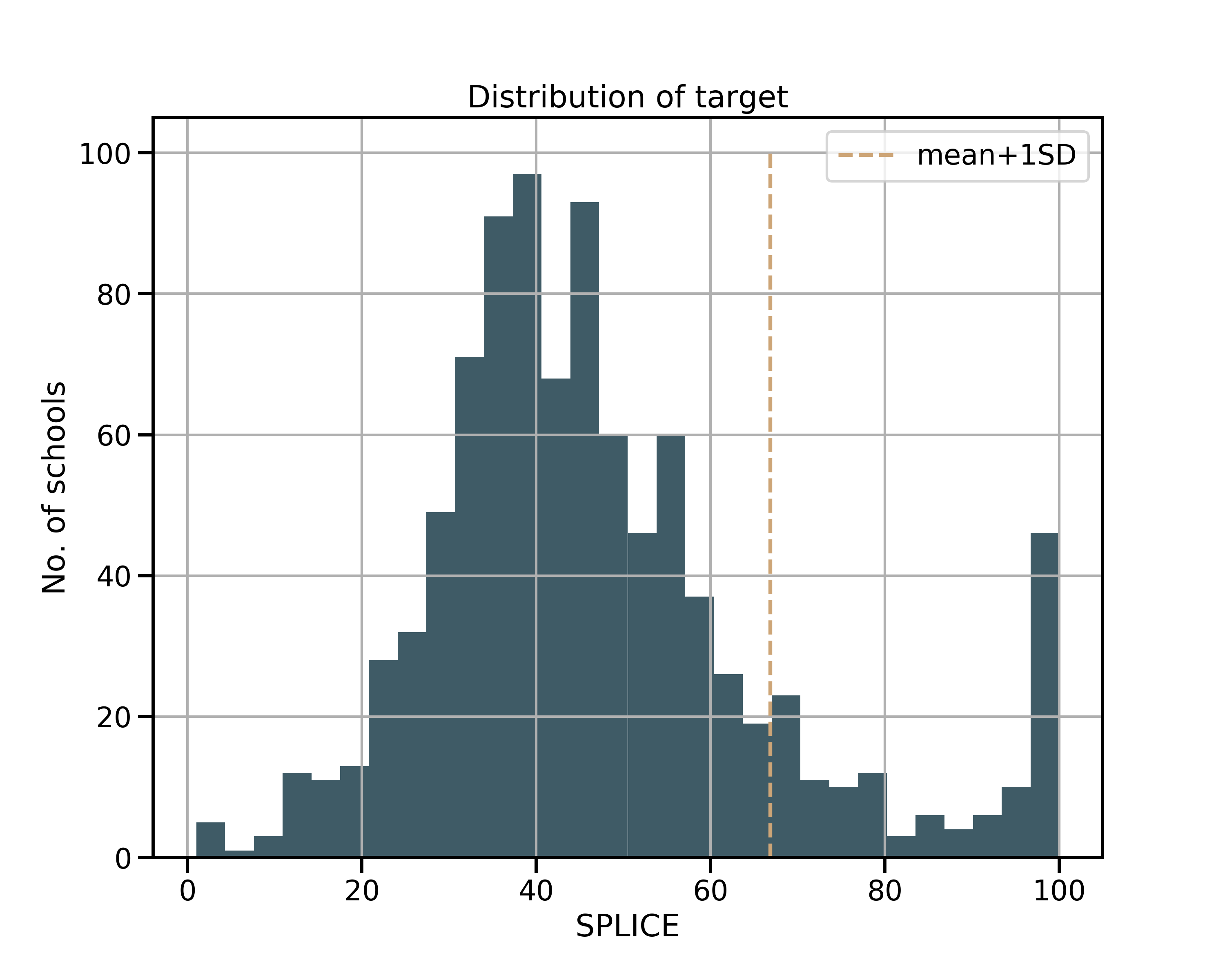
My project questions relied on data sources I could access. While I am interested in understanding success at the student level, obtaining data for individuals was not practical. Some available databases were for schools while community characteristics from census data was at the zip code level. I therefore reframed my questions as “What proportion of low income students at a high school are succeeding?” and “What are the factors associated with that community and school that could drive exceptional success?” My target is a school’s percentage of low income students that are college eligible (SPLICE). Specifically, my target in binary classification models is whether a school shows exceptional SPLICE, with the threshold for exceptional being one standard deviation above mean SPLICE across all CA high schools. The distribution of SPLICE can be seen here:
To be eligible for University of California (UC) or California State University (CSU) colleges, a student must achieve a grade of C or better in two years of history/social science, English (4 years), math (3 years), a laboratory science (2 years), a language other than English (2 years), visual and performing arts (1 year), and a college preparatory elective. This is not an easy bar to clear, regardless of a student’s economic situation. The question of which factors that drive low income student college eligibility is complicated; I am certain that not every possible school and community feature is represented here. But my hope is that a greater understanding of what factors associate with low income student success can facilitate achievement.
Methods
This section provides technical details on how I arrived at the findings but you can skip to the Results.
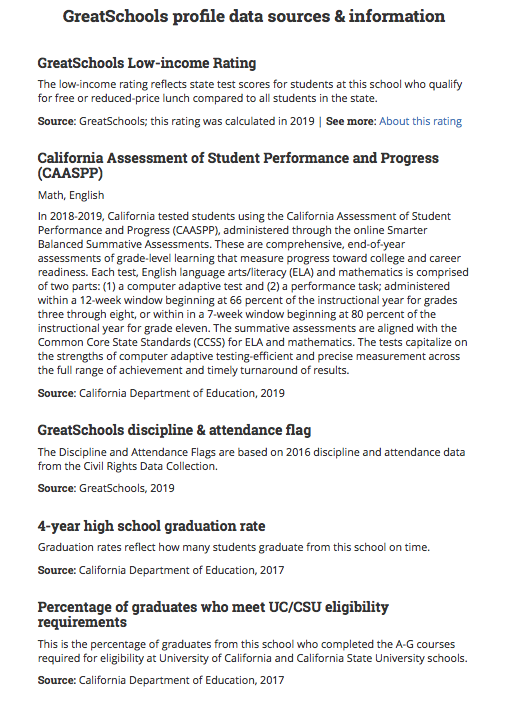
Data collection. Data was collected with Python packages urllib, BeautifulSoup, and xml.tree. The three data sources were (1) the CA Public Schools Database, (2) GreatSchools, and (3) CA economic characteristics from the census on the zip code level. The CA Public Schools database provided information such as name, district, identification numbers, county, address, and enrollment size. Only active, public high schools from this database were included for analysis. Data on GreatSchools sites was used to obtain school-specific performance and staff metrics. An API provided by GreatSchools was used to obtain high-level metrics via an XML tree. Additional metrics, including student-to-counselor ratio, student-to-teacher ratio, average teacher salary, test scores, graduation rates, and the target variable (SPLICE), was acquired by web scraping publicly available sites, which were originally obtained from various sources by GreatSchools. For example, the percent of a school’s low income students that are proficient in English or math come from tests administered through the California Assessment of Student Performance and Progress (CAASPP). California economic characteristics were taken from census data. This includes features of a community for each zip code, including types of industries, income benefits, health insurance status, employment, worker class, and work commute. 401 schools were in the same zip code as at least one other school. Thirty-eight (all in the Los Angeles Unified School District) were co-localized on the same campus as indicated by the street address. After data collection, the dataset consisted of 1110 schools and 264 features. Both figures were reduced in subsequent filtering steps. The CA Public Schools Database and the census data are from 2016 and GreatSchools data sources are from 2016 to 2019. I assumed any temporal differences in this time frame are negligible. Details can be found in the data collection notebook.
Data preprocessing and feature selection. I further filtered the schools and features to improve model robustness and interpretability. Since the focus is on a metric of low-income high school seniors, I only included schools with a minimum of 25 twelfth-graders, of which at least 10 were low income. Features were eliminated if missing values were present in at least one-third of the schools. Additionally, using the Python package statsmodels, I identified and removed features with high variance inflation factor (VIF). High VIF was initially present for many variables if they were a percentage of a category. For example, worker class was represented by multiple features as a percentage of a community where employees were designated as private wage, government, self-employed or unpaid. In this case, the percentage of workers in government were dropped since they were highly anti-correlated with the percentage of workers with private wages and thus VIF decreased. High VIF was also present in correlated features, which were identified by finding the Pearson correlation value or with scatter plots. Most remaining features had a VIF < 10 and the max VIF was 25.2. Additional data preprocessing included feature engineering. I estimated the percentage of non-low-income students that are college eligible from a combination of enrollment data and the percentage of low-income students. Furthermore, ethnic composition of a school by the percentage of underrepresented minorities (African American, American Indian or Hispanic, as indicated here). 966 schools remained following data preprocessing and feature selection. Further information on data preprocessing and feature selection can be found in this notebook.
Data exploration and visualization. For data exploration, I applied Python packages matplotlib and seaborn for univariate and bivariate data visualization, and geopandas and fiona for maps. Geographic reference files came from geojson.xyz and Stanford Earthworks. Details can be found in the data visualization notebook.
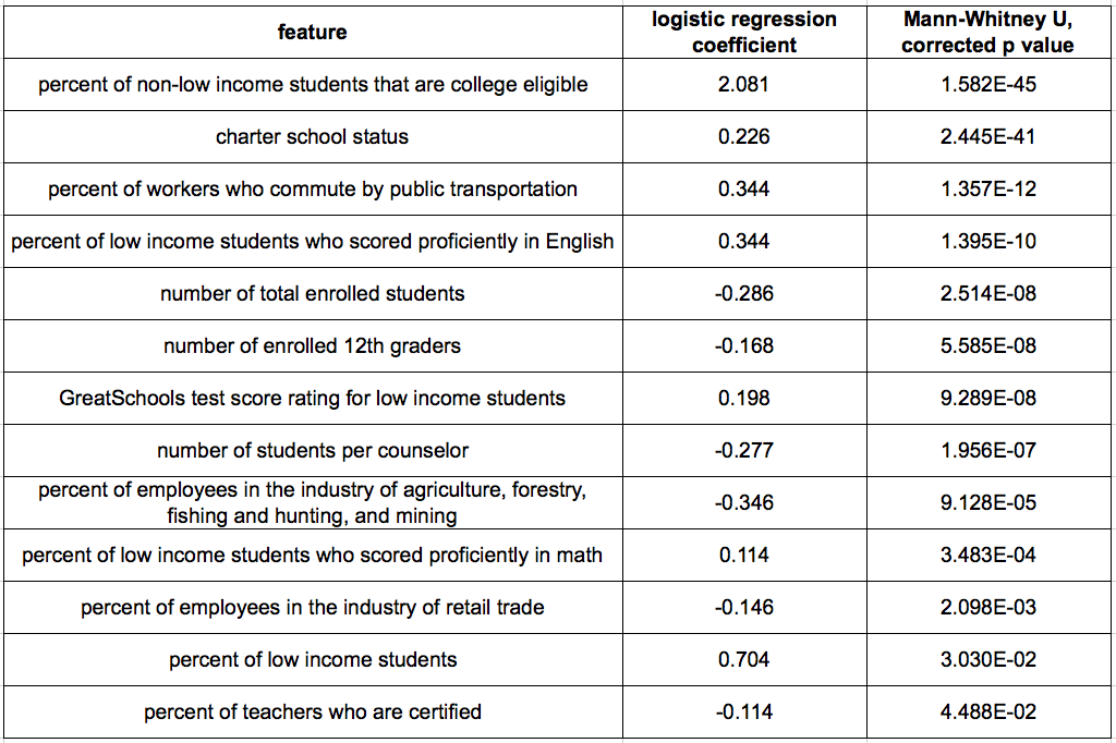
Classification models and statistical analysis. Modeling was performed on the 814 schools that contained no missing values in the 53 features following school and feature filtering. Using scikit-learn, I applied logistic regression (LR) (linear_model.LogisticRegression) and random forest (RF) (ensemble.RandomForestClassifier) to predict exceptional schools for SPLICE. The threshold (66.8%) was defined as one standard deviation above mean for SPLICE across all CA high schools. I applied a 60:20:20 split for train-validation-test. Training-validation employed a 4-fold cross-validation design (model_selection.RandomizedSearchCV) to determine optimal parameters and hyperparameters. The test set was defined as the hold out set for both models with F1 score serving as the primary metric for model evaluation. I applied standardized scaling to the LR model but not in RF where scaling is not necessary. Class weights were run as balanced in both models. LR exhibited a higher F1 for the positive class than RF (see Results). Accordingly, I focused on features interpretability based on LR coefficients. Since RandomizedSearchCV returned L2 regularization for the logistic regression hyperparameters, p-values for the coefficients would not apply. To increase the stringency of features for interpretation and independently of the LR output, I applied a Mann-Whitney U test with Bonferroni correction (statsmodels) to find features that were significantly different between exceptional and non-exceptional schools. I then focused on interpreting features that had a logistic regression coefficient absolute value greater than 0.10 and a corrected p-value from the Mann Whitney U-test of less than 0.05. Further information can be found in the project’s modeling notebook.
Results
Data exploration
Exploration and visualization of data provides context and assists in model interpretability. Here I assessed the geographic representation of schools and the distribution of school and community features before modeling.
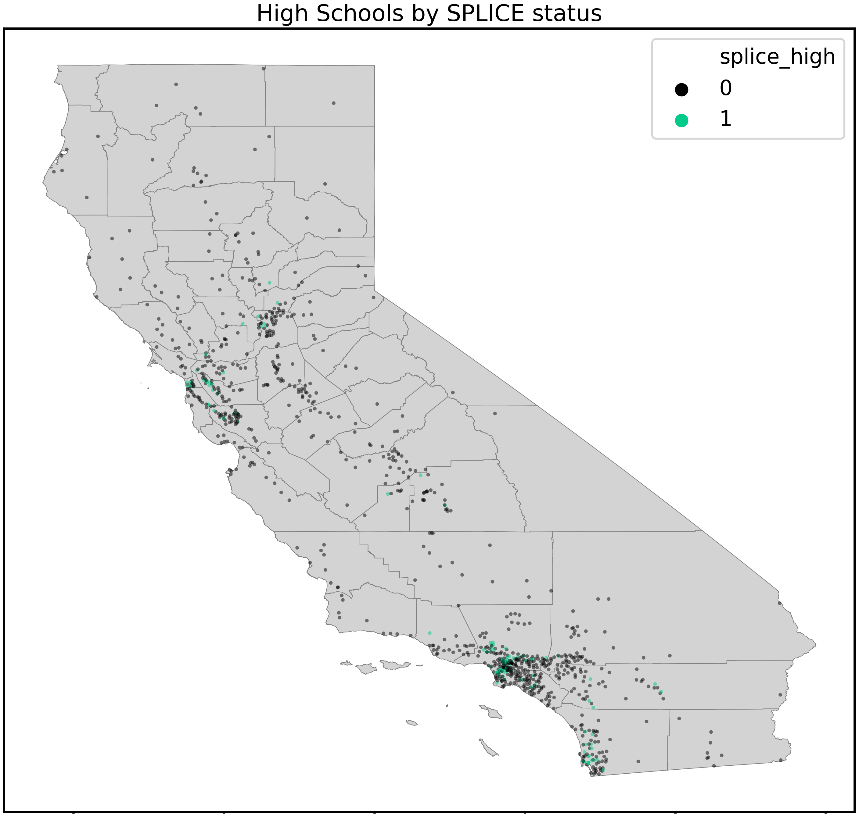
Geographic representation of schools
The dataset contained schools that reflected the state’s population density. The county with the most schools is Los Angeles with 234, which comprised 24.2% of the dataset. Next was San Diego county with 73 schools (7.5% of the data) and Orange County (59 schools). Overall, 55 counties in the state were represented with most (34) represented by fewer than than ten schools in the data. District representation of schools matched the geographic distribution, with the largest Los Angeles Unified (114 schools) having much more than the next largest districts, San Diego Unified (23) and East Side Union High in San Jose (15). Most districts were very small–204 of the 378 districts were represented by only one school.
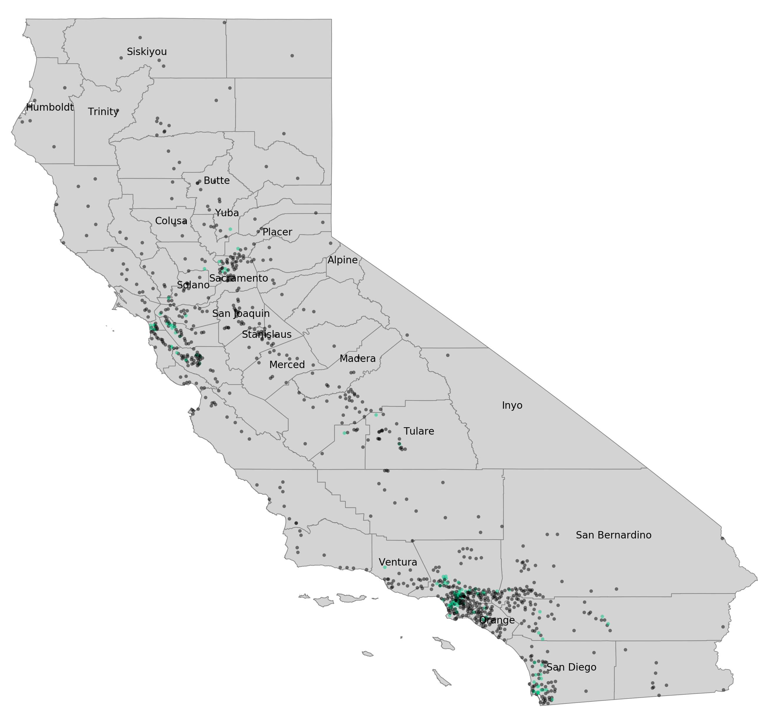
From map inspection and quantitative analysis, most exceptional SPLICE schools were located in the San Francisco Bay Area or Southern California coastal counties (San Diego, Orange, Los Angeles) compared to the rest of the state. These two areas represent 54.1% of schools in the state, but make up 87.0% of CA schools with exceptional SPLICE. This point will be re-visited in the discussion section.
School features
Enrollment was one metric for filtering (see Methods). Out of the remaining schools, the total enrollment average is 1547 but the standard deviation of 897 is an indication of high size variablity. The smallest school had 90 students (Round Valley High in Mendocino County) while the largest enrolled 8000 (Opportunities for Learning - Baldwin Park). Interestingly, distribution of total enrollment and the number of enrolled seniors shows bimodality.
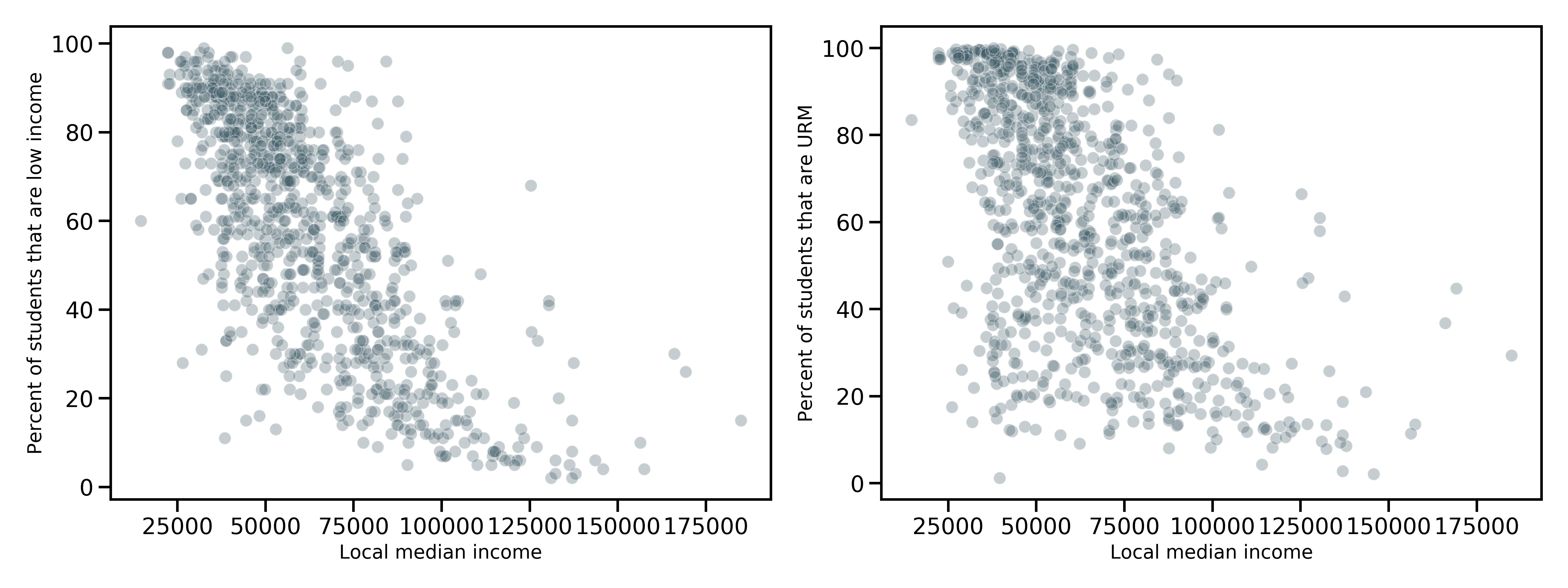
With regards to student demographics, the average percentage of under-represented minorities is 60% (SD 27.5%) and the percentage of low-income students was 57% (SD 25.7%). The correlation between these two metrics was high (Pearson r of 0.86).
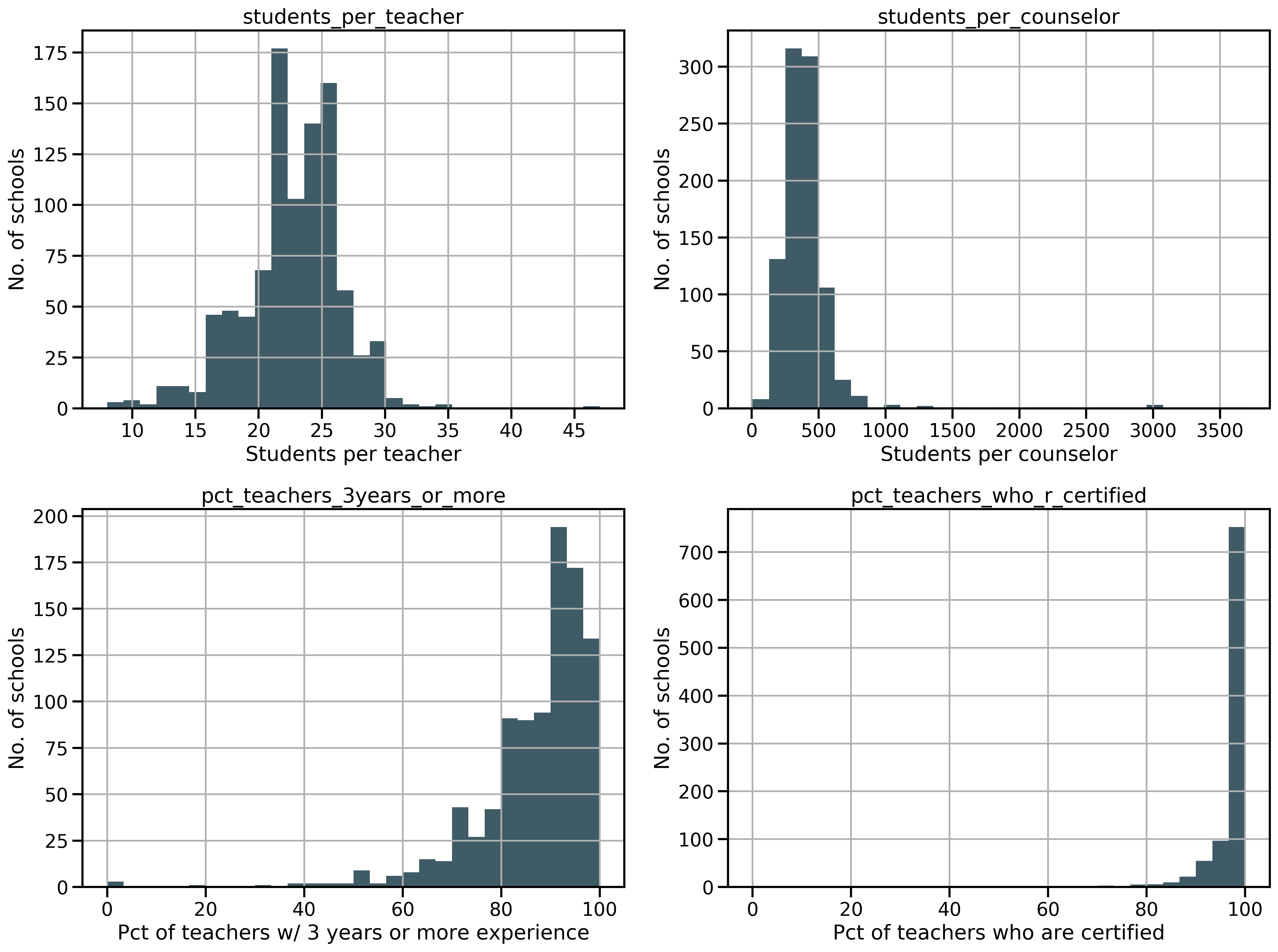
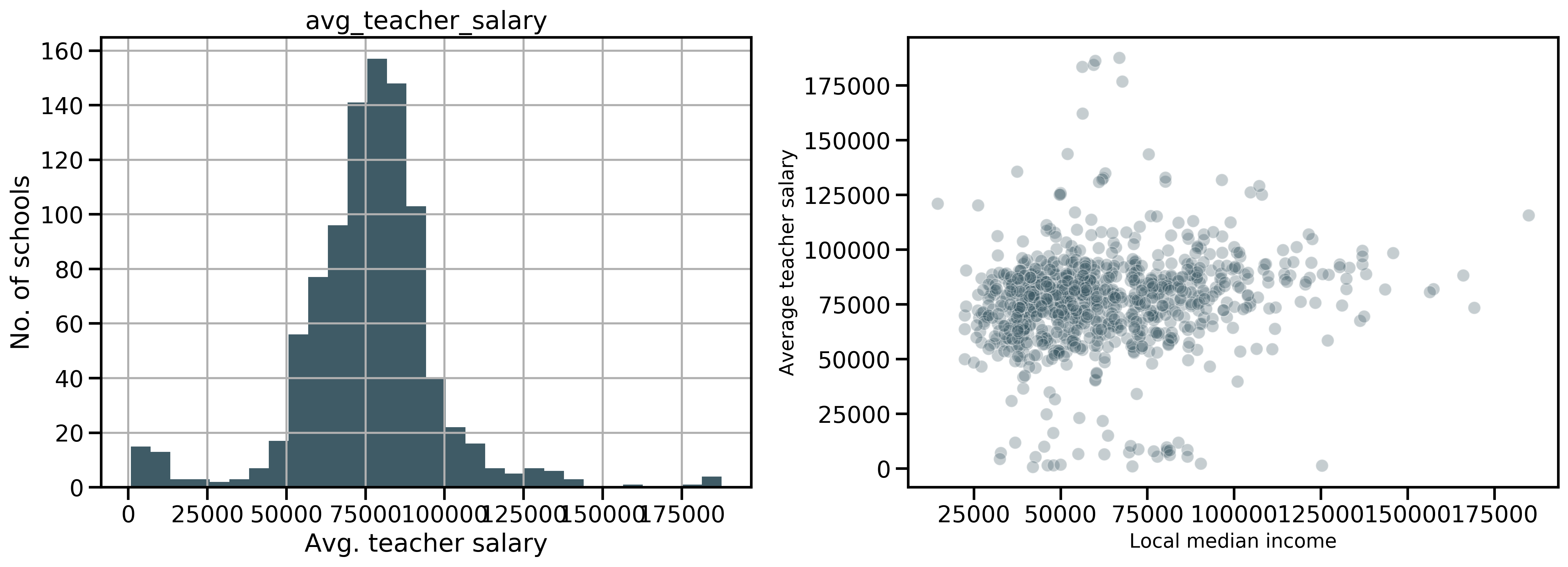
Features related to staff included the number of students per teacher (23 +/- 3.9), number of students per counselor (408 +/- 267.5), the percentage of teachers with 3 or more years of experience (87 +/- 12.0) and the percent of teachers who are certified (98 +/- 5.6). The latter two have left-skewed distributions. Teacher salary averaged $76,200 (SD $22,250) and correlated weakly with a community’s local median income (Pearson r of 0.15).
119 schools in the set were designated as a charter school and 99 were magnet; five schools were both magnet and charter.
Community features
Census information at the level of zip codes provided insight on an area’s income benefits, industries, health insurance status, employment, worker class, and work commute.
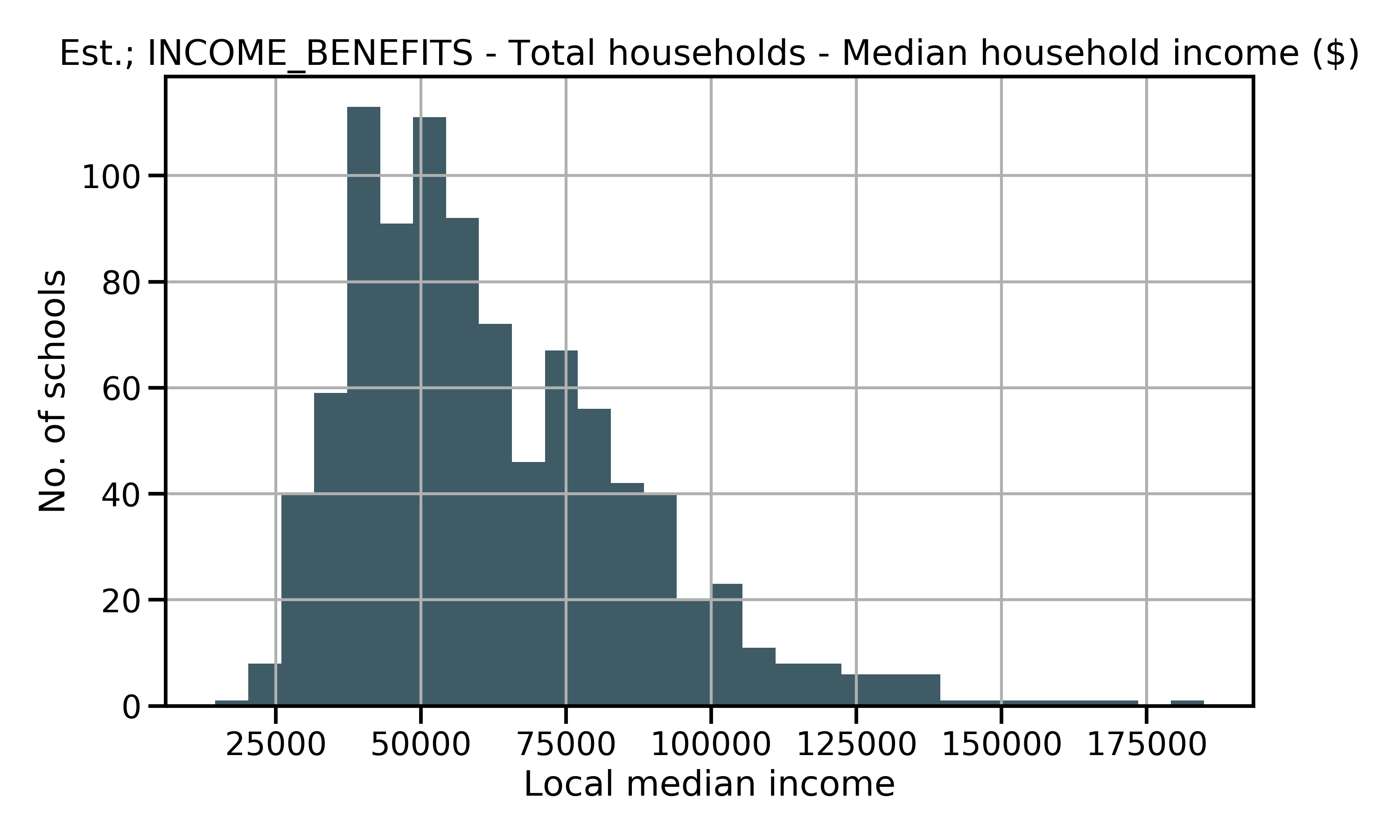
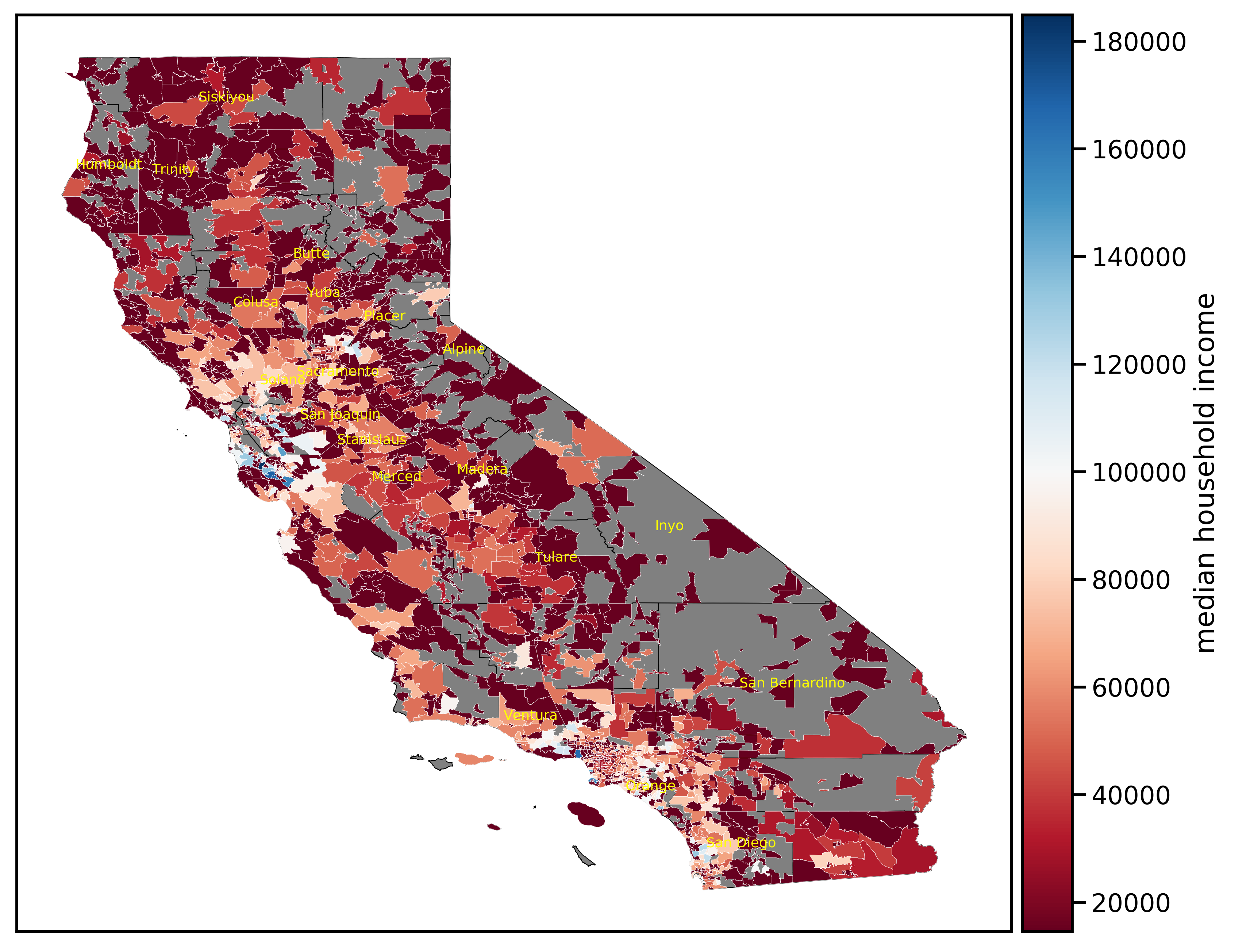
Local median income averaged $62,520 (SD of $24,807) across all communities in the dataset. The distribution shows right skewness demonstrating few areas in the upper ends of income levels. A map of income levels further highlights the striking variability.
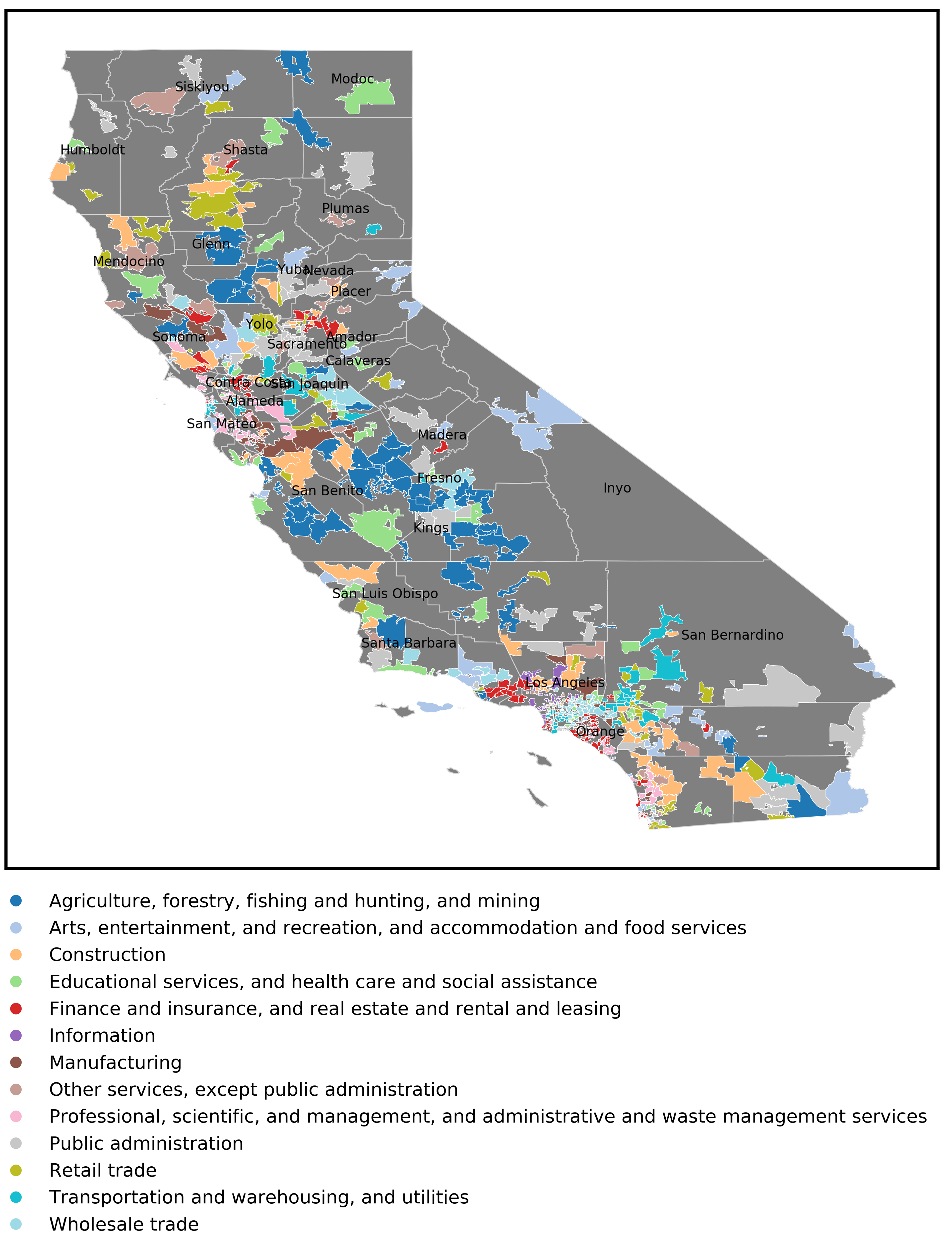
I also looked at industries that are significantly represented in a given area, acknowledging that all communities must have a diverse set of occupations. I first determined the mean and standard deviation of the percent of workers in each industry category across the dataset. This was followed by calculating the z-statistic for each category and zip code. The industry category with the highest z-statistic for that community was then assigned as representative. Only areas where schools were in the dataset were plotted.
Data exploration and additional details on income benefits, industry, health insurance status, employment, worker class, and work commute features can be found in the data visualization notebook. Some community features are discussed further below.
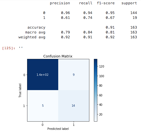
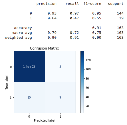
Model performance for predicting schools with exceptional SPLICE
Given that predicting schools with exceptional SPLICE is a binary classification problem, I employed logistic regression (LR) and random forest (RF) classification. LR models the probability that a school will be exceptional for SPLICE and learns coefficients associated with each feature. A positive coefficient represents the log odds of the school being exceptional by a one-unit increase in the feature, while a negative coefficient decreases the association of the feature with the school being exceptional. (All features were standardized for comparison.) RF uses an ensemble of decision trees. Each tree only uses a subset of predictors, decorrelating the trees making the average of the resulting trees more reliable.
While I assessed multiple evaluation metrics, I optimized for F1 score for both data science and potential decision-making reasons. Schools with exceptional SPLICE are a small class and assessing F1 of the positive class accounts for both false positives (predicting a school with exceptional SPLICE when it is not) and false negatives (predicting a school that is not exceptional for SPLICE when it is). Predictions without false calls would have an F1 score of 1. From a policy perspective, minimizing both types of false predictions is important since the main objective is identifying important school or community features of exceptional SPLICE. Both models performed well for predicting schools that would not be exceptional (F1 of 0.95 for both LR and RF, respectively). However, LR outperformed RF on recall and F1 for the positive class. The LR model achieved an F1 score of 0.67 while the RF F1 score was 0.55 for predicting exceptional schools. Due to model performance, I prioritized features identified by logistic regression instead of by random forest. To further increase the stringency of variables for interpretation, I applied two-sample statistical testing (Mann-Whitney U with Bonferroni correction) independently of modeling and on the same set of features. I identified those that were significantly different between exceptional and non-exceptional schools. In the next section, I discuss the features with logistic regression coefficients greater than 0.10 (by absolute value) and a corrected p-value from the Mann Whitney U-test of less than 0.05 (see Methods). The thirteen features that matched this criteria are shown in Table 1:
School and community features of exceptional SPLICE
School features important in exceptional SPLICE prediction: student population, school size, charter status, and staff characteristics
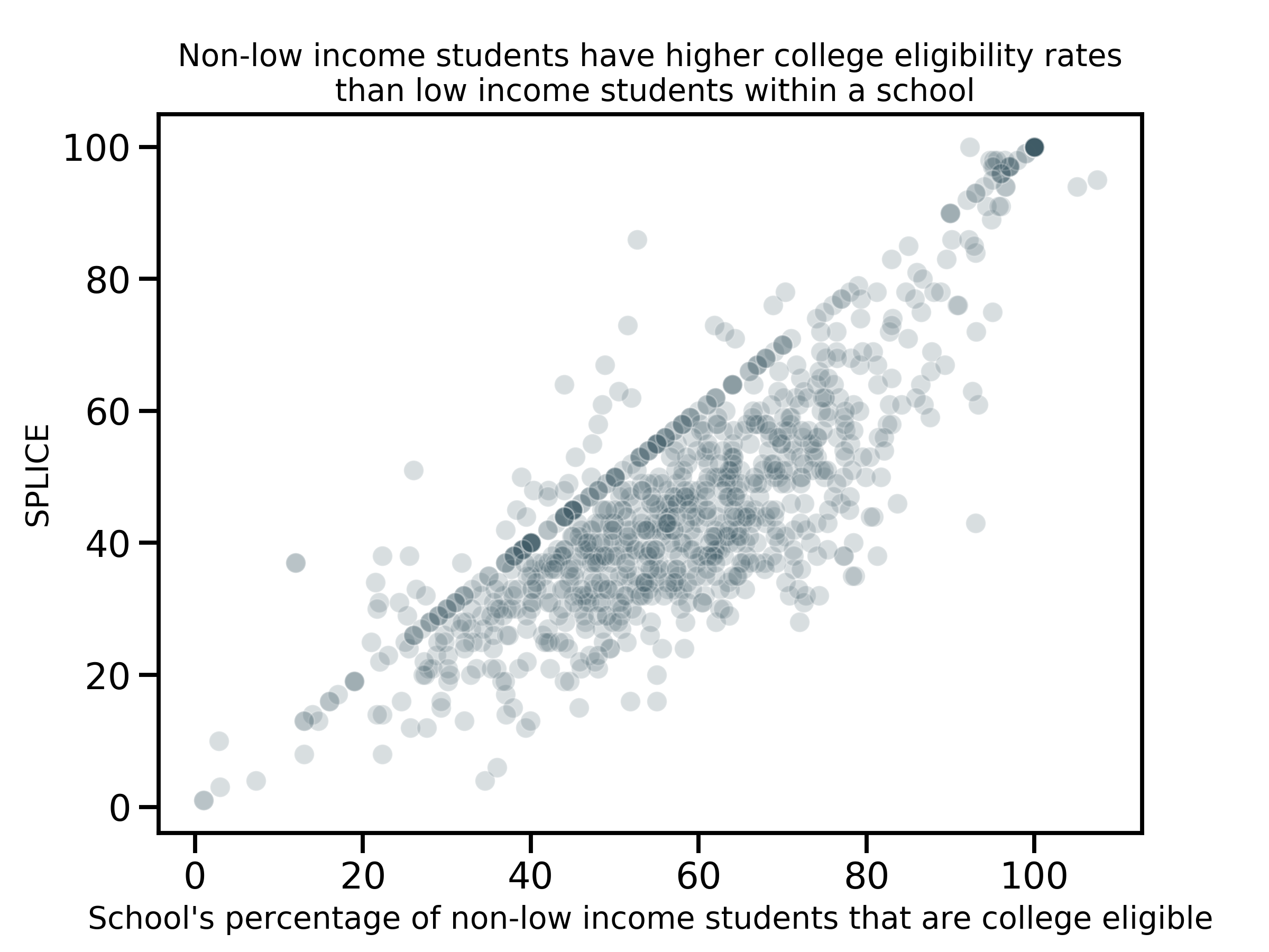
Student population and test performance. By far, the top feature with exceptional SPLICE, is the percentage of non-low income students who are college eligible. This feature is positively associated with SPLICE suggesting that academic environments provide benefits across the socioeconomic spectrum of their students. However, a gap between non-low income students and low income students within a school for college eligibility is still prevalent. A school’s percentage of low-income students (regardless of college eligibility) was not correlated with SPLICE overall, but it was positively associated in predicting schools with exceptional SPLICE. In addition, while the percent of low income students that have tested for both English proficiency and math proficiency were positively associated with exceptional SPLICE, the percentage of low income students that scored proficiently in English had a higher coefficient, suggesting that it provides a better prediction of the target.
School size. Interestingly, smaller schools, but not necessarily smaller class sizes, are common in schools of exceptional SPLICE. Features indicative of overall school size, such as number of enrolled 12th graders (E12), enrollment, and student-per-counselor ratio were negatively associated with exceptional SPLICE. However, the ratio of student-per-teacher did not necessarily need to be small and, in fact, shows a small positive correlation with schools that performed highly for SPLICE.
Charter/magnet status. A charter school positively associated with exceptional SPLICE. (This feature was also the second-most significant feature by the Mann-Whitney test). Magnet school status was not predictive of exceptional SPLICE.
Staff characteristics. An unexpected finding with regards to staff features is that schools with exceptional SPLICE tended to have a lower percentage of teachers who are certified, especially since this metric is heavily left-skewed. Non-significant features to the model also included the percent of teachers who have 3 or more years of experience and average teacher salary, suggesting that schools with exceptional SPLICE do not necessarily have the most experienced and best paid teachers.
Community features of a school associated with exceptional SPLICE prediction
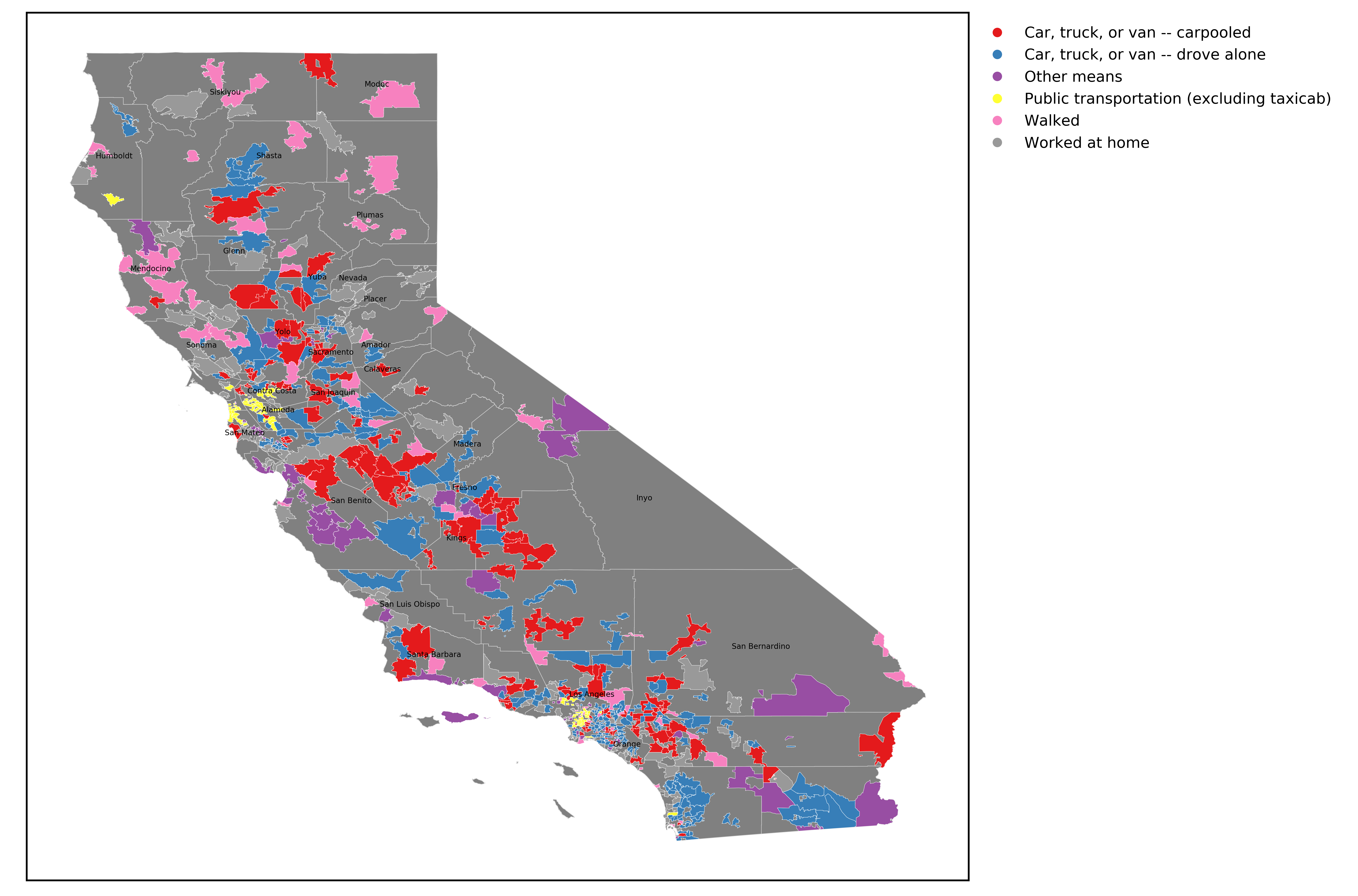
Economic characteristics of a school’s community is taken from census data. This data was obtained at the zip code level and not directly from the associated school population. This means that students and their families may live in one zip code and attend schools or work in another zip code. With these caveats noted, the assumption is that the features are largely reflective of the community. One observation from the analysis is that schools with exceptional SPLICE are in an area where many workers commute by public transportation instead of driving alone. Exceptional SPLICE schools were also negatively associated with communities where the predominant industry involved agriculture, forestry, fishing and hunting, and mining or retail trade. This is reflective of the locations of schools with exceptional SPLICE and an area’s predominant industry. I would like to emphasize that correlation does not imply causation and I have more to say about this result in the discussion.
Features that had low predictive value by logistic regression or not significant by two-sample statistical testing
Most features related to income benefits (local median income, percent of community receiving supplemental security income, etc.) were not predictive, but a percent of a community receiving social security benefits had a significant Mann Whitney U p-value and logistic regression coefficient of -0.094 (just under the 0.10 absolute value threshold). Most features related to health insurance coverage (percent of community with public health insurance coverage and percent of children without health insurance coverage) were not predictive or significantly different. Interestingly, for the percentage of a community with health insurance, the Mann Whitney U test shows no statistical significance between the negative and positive classes for exceptional SPLICE but the logistic regression coefficient was -0.30. Magnet schools were not positively or negatively associated with exceptional SPLICE. Ethnic composition of a school, represented as the percent of under-represented minorities, had a LR coefficient of 0.239 but was not significant by Mann Whitney U.
Discussion: Placing the results in context
I initiated this project because I wondered, “Where are places where low income students are succeeding exceptionally? What do those communities look like?” Focusing on my home state of California, I gained some answers. But I only see this as a starting point of a discussion, one made more difficult with the cancellation of in-person conferences during the pandemic. (Since posting this article, I reached out to my network and started to document feedback from educators.) It is natural to ask whether some of these findings can be called “causes.” But without context, this is a dangerous exercise. It is easy to misconstrue some of these findings, hence the pre-emptive cautionary note at the start of this article.
Before we can think about the implications of the results, I stress that the models I used to predict schools of exceptional SPLICE did not show great performance and nor did I necessarily expect them to. One immediate explanation is that not every feature of a school or community is captured here. (This would be very difficult to do even if that was the aim.) And for those variables that are in the model, most are insignificant or contribute only a small amount to the prediction.
Acknowledging the study imperfections, and with proper context, for what results can we consider implications or generate new questions? It is reasonable to wonder which features might matter and where. One finding is that schools that are in a community where a high proportion of workers commute by public transportation is positively associated with exceptional SPLICE. Perhaps public transportation may ease the burden on workers to drive their kids to school. This idea has been voiced in some proposals with respect to facilitating student access to colleges. The importance of alternatives to driving to schools makes sense in areas of high population density. But does this mean we should encourage more Shasta County employees to start taking the bus? Of course not. Likewise, it is ridiculous to think that changing an area’s industry from one that has a negative association with SPLICE to one that is positive would increase the number of exceptional SPLICE schools. However, I think it is reasonable to look into why exceptional SPLICE schools are less prevalent outside the Bay Area and Southern CA coastal counties. I am certainly curious about this. If anything, this suggests that attention should be given towards low income students living in the less population dense parts of the state, while maintaining and improving successful efforts in the metropolitan areas.
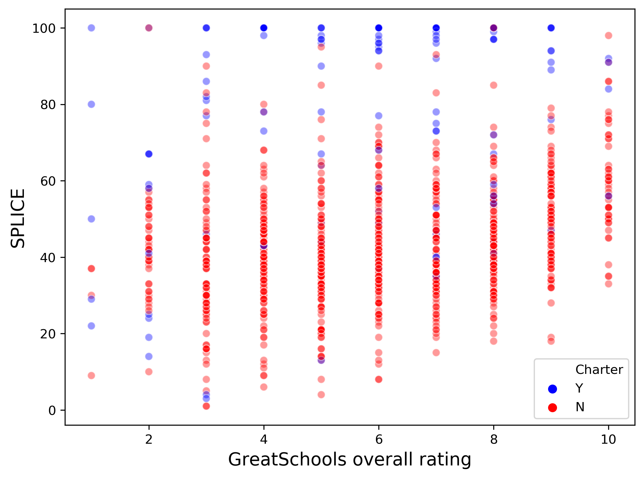
Another important feature that can use additional examination is charter school status. Charter schools are publicly funded, independently run alternatives to traditional public schools. It is not within the scope of this study to understand what characteristics of charter schools contribute to the prediction of exceptional SPLICE. Others have pointed out that charters have more autonomy in tailoring curricula to students, especially within urban settings (see here and here). However, charter schools are not without controversy. Like all schools, they can vary in quality. They also may compete with traditional public school resources, even sharing the same campus. (As noted in the Methods, 38 schools in the Los Angeles Unified School District share an address with another school). Charter schools have certainly demonstrated success in terms of SPLICE, but evaluating together with GreatSchools ratings show a more nuanced picture.
Other features identified as important for a school with exceptional SPLICE line up with other studies or intuition. For example, the highest coefficient in the LR model was associated with the college eligibility rates of less disadvantaged students. This is to not ignore the gap between non-low income and low income students in overall college eligibility rate, but this suggests that academic environments that influence the performance of one group generally applies to another. In addition, exceptional SPLICE is associated with smaller schools. Even though student-to-teacher ratio was not an important feature in the prediction, it is reasonable to assume that an individual student has more support when a school has fewer students overall. This is consistent with the study’s finding that exceptional SPLICE was more likely when the number of students per counselor was smaller (student-to-counselor ratio was negatively associated with exceptional SPLICE). Interestingly, one of the recommendations to help low income students suggested by GreatSchools is to offer college counseling. Moreover, it makes sense that a school’s percentage of low income students that are proficient in English and math, based on the CAASPP assessments, would also be predictive of exceptional SPLICE. It is interesting that SPLICE prediction is slightly better with English proficiency than math. An argument can be made that a student’s aptitude in English might be a bit more important than math when inspecting the subject requirements for UC/CSU eligibility.
Some results lead to additional questions, especially about variables that were not significant or in an unexpected direction with exceptional SPLICE. One feature that I thought would be predictive is local median income. I guessed that wealthier areas would have the resources to better support a low income student: the correlation is small but teachers are slightly better paid when local incomes are higher and a low income student could get more attention since there would be a lower percentage of students are low income or minority. But the analysis here does not support the hypothesis that an exceptionally higher percentage of low income students perform academically better in schools located in high income areas. Counterintuitively, the percentage of low income students itself was a positive predictor of exceptional SPLICE. Why is that? And why would schools with exceptional SPLICE be more likely to have teachers on staff that are not certified? I don’t have an answer to these questions.
No matter the findings reported here, we can certainly say that the factors that contribute to exceptional SPLICE are, well, complicated. Additional questions that one could ask are: What are students’ home lives like? Is there a selection process just for enrollment? What kind of tutoring services are available to students outside of school? What kind of access do they have to the internet and technology? What is the variability in teacher quality?
The questions of what it takes to support low income students to succeed academically cannot be fully addressed here. As I have stated above, I am interested in discussing the results in collaboration with others, especially teachers. A New York Times article appeared recently that asked educators Do children’s zip codes at birth determine their futures? Some of the teachers interviewed share are similar to what this project has found. Some are different or new. But all voice concern about the challenges of poverty. As if low-income students do not deal with enough challenges, Covid-19 has prompted some efforts to re-route funding away from low-income districts.
Continuing to probe what factors help low income students succeed and implementing those that make a difference will help address an important societal challenge.
Acknowledgements
While this project was started before my Insight Data Science Fellowship, I thank the Insight SV 20A cohort for their teachings, feedback, code sharing, and support as I updated and finished this study. I am also grateful to my wife for her feedback and encouragement in posting this article. Finally, I appreciate in advance other questions and comments. I can be reached at ben.lacar AT gmail.com. Feedback from educators and those that work with low income students will be shared here with permission.
The project repository contains Jupyter notebooks where additional figures can be found. This article was first posted on this blog on May 25, 2020. It was last updated on June 11, 2020. Updates thus far have been for grammatical edits, clarity, or figure improvements and not to changes in the main results.