Instrumental variable analysis with a binary outcome
Here is an additional post on instrumental variable (IV) analysis. This follows an exercise where I employed two methods of IV analysis, comparing a Bayesian approach with two-stage least squares (2SLS). My motivation for these posts is to have a better understanding, ultimately, of Mendelian randomization. The context in which I ultimately want to apply it to is a disease outcome, which is binary. In this post, I explore the Bayesian approach of IV analysis towards a binary outcome.
import arviz as az
import matplotlib.pyplot as plt
import numpy as np
import pandas as pd
import pymc as pm
import pytensor.tensor as pt
import scipy.stats as stats
import seaborn as sns
from scipy.special import expit
from utils import draw_causal_graph, standardize
RANDOM_SEED = 73
np.random.seed(RANDOM_SEED)
sns.set_context("talk")
sns.set_palette("colorblind")
cb_palette = sns.color_palette()
Notes
- check p per subject
- model, binary outcome, variable n
Causal graph of example dataset with binary outcome
We’ll return to the wages and education example from Chapter 14 of Statistical Rethinking. However, instead of using wages as our outcome, we’ll tweak this by creating a binary outcome from wages, which I’ll refer to as $R$ for “rich”. The causal diagram will look the same as a traditional IV setup.
draw_causal_graph(
    edge_list=[("Q", "E"), ("U", "E"), ("U", "R"), ("E", "R")],
    node_props={"U": {"style": "dashed"}},
    graph_direction="TD",
)

Per usual, we’ll use this to generate a simulated dataset. We’ll use the same code but this time derive R from W. The rationale being those with higher wages are more likely to be rich. We’ll still making the influence of education on wages (bEW_sim) equal to 0. We’ll want to get this value back in our statistical models, even though we’ll be using R as our ultimate outcome variable.
A key conceptual point is use of a logit link function to produce R from W. Additionally, we’ll make use of a binomial generalized linear model.
def generate_data(num_subjects, n_binomial_param) -> pd.DataFrame:
    """Generate simulated data.

    Parameters
    ----------
    num_subjects
        Number of subjects/rows in data
    n_binomial_param
        Number of "observations" for each subject;
        a parameter in the binomial GLM

    Returns
    -------
    sim_df
        pd.DataFrame

    """

    bEW_sim = 0

    U_sim = np.random.normal(size=num_subjects)
    Q_sim = np.random.randint(1, 5, size=num_subjects)
    E_sim = np.random.normal(loc=U_sim + Q_sim, size=num_subjects)
    W_sim = np.random.normal(loc=U_sim + bEW_sim * E_sim, size=num_subjects)
    sim_df = pd.DataFrame.from_dict(
        {"W": standardize(W_sim), "E": standardize(E_sim), "Q": standardize(Q_sim)}
    )

    # Use of link functions to generate R
    index_val = sim_df.index.values
    sim_df["R"] = stats.binom.rvs(n=n_binomial_param, p=expit(W_sim))
    sim_df["R_size"] = n_binomial_param

    return sim_df


dat_sim = generate_data(num_subjects=500, n_binomial_param=2)
dat_sim.head()
| W | E | Q | R | R_size | |
|---|---|---|---|---|---|
| 0 | -1.327032 | -0.600469 | 0.453638 | 1 | 2 |
| 1 | -0.108554 | -0.159673 | -1.318387 | 0 | 2 |
| 2 | -0.908108 | 1.066808 | 0.453638 | 2 | 2 |
| 3 | -2.187143 | -2.856829 | -1.318387 | 0 | 2 |
| 4 | 0.044873 | -0.024763 | -0.432374 | 1 | 2 |
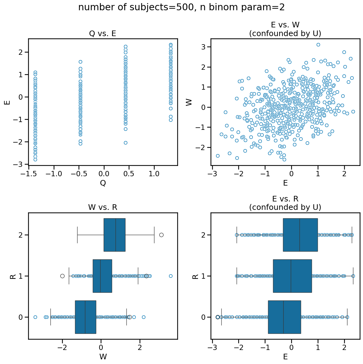
As usual, visualizing the data can give us some insight into how the data appears and where confounds may mislead. We know that Q is a cause of E and therefore the association we see is reflective of causation. The bottom-left figure W vs. R is a logit transformation of the former into the latter. However, both the plots in the right column are a result of the confound U. It is driving the relationship between E and W and therefore we also see an association between E and R.
def plot_variable_relationships(sim_df, title):
    f, ((ax0, ax1), (ax2, ax3)) = plt.subplots(2, 2, figsize=(12, 12))

    sns.scatterplot(data=sim_df, x="Q", y="E", marker=r"$\circ$", ax=ax0)
    ax0.set_title("Q vs. E")

    sns.scatterplot(data=sim_df, x="E", y="W", marker=r"$\circ$", ax=ax1)
    ax1.set_title("E vs. W\n(confounded by U)")

    sns.boxplot(data=sim_df, x="W", y="R", orient="h", color=cb_palette[0], ax=ax2)
    sns.scatterplot(data=dat_sim_n1, x="W", y="R", marker=r"$\circ$", ax=ax2)
    ax2.invert_yaxis()
    ax2.set_title("W vs. R")

    sns.boxplot(data=sim_df, x="E", y="R", orient="h", color=cb_palette[0], ax=ax3)
    sns.scatterplot(data=sim_df, x="E", y="R", marker=r"$\circ$", ax=ax3)
    ax3.invert_yaxis()
    ax3.set_title("E vs. R\n(confounded by U)")

    f.suptitle(title)
    f.tight_layout()


plot_variable_relationships(dat_sim, "number of subjects=500, n binom param=2")
Bayesian model with binary outcome
We’ll use the Bayesian approach to run our inferential model. Again, the important thing is the link function to get our count output.
\[R_i \sim \text{Binomial}(n_i, p_i)\] \[\text{logit}(p_i) = W_i\] \[\left( \begin{array}{c} W_i \\ {E_i} \end{array} \right) \sim \text{MVNormal} \left( \begin{array}{c}{\mu_{W_i}} \\ {\mu_{E_i} } \end{array} , \textbf{S} \right)\] \[\mu_{W_i} = \alpha_W + \beta_{EW} W_i\] \[\mu_{E_i} = \alpha_E + \beta_{QE} E_i\] \[\alpha_W, \alpha_E \sim \text{Normal}(0, 0.2)\] \[\beta_{EW}, \beta_{QE} \sim \text{Normal}(0, 1.5)\] \[\textbf{S} = \begin{pmatrix} \sigma_{W}^2 & \rho\sigma_{W}\sigma_{E} \\ \rho\sigma_{W}\sigma_{E} & \sigma_{E}^2 \end{pmatrix} = \begin{pmatrix} \sigma_{P} & 0 \\ 0 & \sigma_{\beta} \end{pmatrix} \textbf{R} \begin{pmatrix} \sigma_{W} & 0 \\ 0 & \sigma_{E} \end{pmatrix}\] \[\textbf{R} \sim \text{LKJCorr}(2)\]def run_bayesian_iv_model_binary(data_df):
"""Model for education/rich binary outcome.
Parameters
----------
data_df
Generated dataset
Returns
-------
:
pymc idata object
"""
index_vals = data_df.index.values
with pm.Model() as model:
aW = pm.Normal("aW", 0.0, 0.2)
aE = pm.Normal("aE", 0.0, 0.2)
bEW = pm.Normal("bEW", 0.0, 0.5)
bQE = pm.Normal("bQE", 0.0, 0.5)
muW = pm.Deterministic("muW", aW + bEW * data_df.E.values)
muE = pm.Deterministic("muE", aE + bQE * data_df.Q.values)
chol, _, _ = pm.LKJCholeskyCov(
"chol_cov", n=2, eta=2, sd_dist=pm.Exponential.dist(1.0), compute_corr=True
)
# multivariate regression
MU = pt.stack([muW, muE]).T
YY_obs = pm.Data("YY_obs", data_df[["R", "E"]].values)
YY = pm.MvNormal("YY", mu=MU, chol=chol, observed=YY_obs)
# link function
p = pm.Deterministic("p", pm.math.invlogit(YY[index_vals, 0]))
R = pm.Binomial("R", n=data_df["R_size"], p=p, observed=data_df["R"])
idata = pm.sample(1000, random_seed=RANDOM_SEED, target_accept=0.95)
idata.rename({"chol_cov_corr": "Rho", "chol_cov_stds": "Sigma"}, inplace=True)
return idata
idata_14_6_logit = run_bayesian_iv_model_binary(dat_sim)
Sampling 4 chains, 0 divergences ━━━━━━━━━━━━╸━━━━━━━━━━━━━━━━━━━━━━━━━━━ 32% 0:00:17 / 0:00:10
IOPub message rate exceeded.
The Jupyter server will temporarily stop sending output
to the client in order to avoid crashing it.
To change this limit, set the config variable
`--ServerApp.iopub_msg_rate_limit`.

Current values:
ServerApp.iopub_msg_rate_limit=1000.0 (msgs/sec)
ServerApp.rate_limit_window=3.0 (secs)
Sampling 4 chains for 1_000 tune and 1_000 draw iterations (4_000 + 4_000 draws total) took 48 seconds.
f, ax0 = plt.subplots(1, 1, figsize=(6, 5), sharex=True)
az.plot_forest(idata_14_6_logit, var_names=["bEW", "bQE"], combined=True, ax=ax0)
ax0.set_title("m14.6 with logistic link")
Text(0.5, 1.0, 'm14.6 with logistic link')
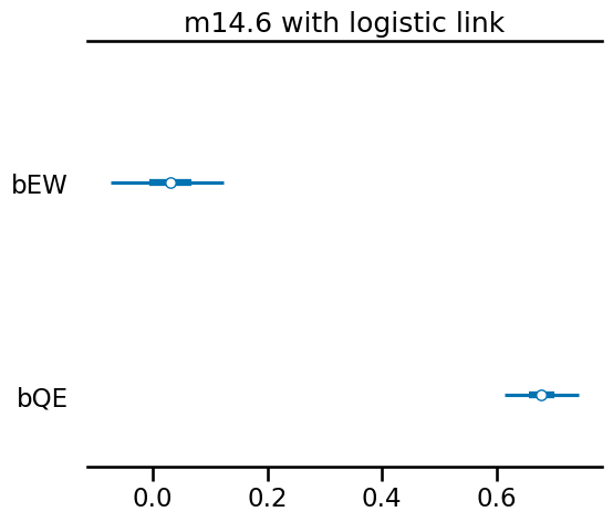
As you can see, we get coefficients as the original wages and education example.
Experimenting with number of subjects and the binomial parameter
A practical question we might have in a real world scenario is how many subjects we might need and how many observations we might want per person. Generally, more people will give us more power for our estimate. We can run experiments to help us understand how these parameters influence the credible interval of our estimate.
num_subjects_list = [25, 100, 200, 500]
n_binomial_param_list = [1, 2, 5]
def format_summary_table(
    idata, num_subjects, n_binomial_param, var_names=["bEW", "bQE"]
):
    df = (
        az.summary(idata, var_names=var_names)
        .assign(num_subjects=num_subjects)
        .assign(n_binomial_param=n_binomial_param)
    )
    return df
df_summary = list()
for num_subjects in num_subjects_list:
    for n_binomial_param in n_binomial_param_list:
        print(
            f"Running {num_subjects} num_subjects, {n_binomial_param} n_binomial_param..."
        )
        dat_sim_expt = generate_data(
            num_subjects=num_subjects, n_binomial_param=n_binomial_param
        )
        idata_14_6_logit_expt = run_bayesian_iv_model_binary(dat_sim_expt)
        df_expt_summary = format_summary_table(
            idata_14_6_logit_expt,
            num_subjects=num_subjects,
            n_binomial_param=n_binomial_param,
        )
        df_summary.append(df_expt_summary)

print("Done with experiment")
df_summary = pd.concat(df_summary)
df_summary
| mean | sd | hdi_3% | hdi_97% | mcse_mean | mcse_sd | ess_bulk | ess_tail | r_hat | num_subjects | n_binomial_param | |
|---|---|---|---|---|---|---|---|---|---|---|---|
| bEW | 0.254 | 0.163 | -0.067 | 0.556 | 0.005 | 0.003 | 1330.0 | 1345.0 | 1.0 | 25 | 1 |
| bQE | 0.430 | 0.174 | 0.087 | 0.741 | 0.003 | 0.002 | 3144.0 | 2492.0 | 1.0 | 25 | 1 |
| bEW | 0.075 | 0.290 | -0.491 | 0.606 | 0.007 | 0.005 | 1558.0 | 1779.0 | 1.0 | 25 | 2 |
| bQE | 0.572 | 0.158 | 0.256 | 0.841 | 0.003 | 0.002 | 2945.0 | 2536.0 | 1.0 | 25 | 2 |
| bEW | -0.118 | 0.447 | -1.018 | 0.664 | 0.009 | 0.007 | 2226.0 | 2858.0 | 1.0 | 25 | 5 |
| bQE | 0.503 | 0.153 | 0.203 | 0.777 | 0.003 | 0.002 | 2942.0 | 2430.0 | 1.0 | 25 | 5 |
| bEW | 0.069 | 0.077 | -0.078 | 0.212 | 0.002 | 0.001 | 2062.0 | 1784.0 | 1.0 | 100 | 1 |
| bQE | 0.631 | 0.078 | 0.491 | 0.780 | 0.001 | 0.001 | 4154.0 | 3071.0 | 1.0 | 100 | 1 |
| bEW | 0.097 | 0.134 | -0.157 | 0.339 | 0.003 | 0.002 | 1835.0 | 1786.0 | 1.0 | 100 | 2 |
| bQE | 0.589 | 0.079 | 0.442 | 0.736 | 0.001 | 0.001 | 2903.0 | 2622.0 | 1.0 | 100 | 2 |
| bEW | -0.723 | 0.394 | -1.434 | 0.028 | 0.012 | 0.009 | 1025.0 | 1450.0 | 1.0 | 100 | 5 |
| bQE | 0.555 | 0.087 | 0.389 | 0.718 | 0.002 | 0.002 | 1328.0 | 2054.0 | 1.0 | 100 | 5 |
| bEW | -0.026 | 0.055 | -0.129 | 0.077 | 0.001 | 0.001 | 2076.0 | 2150.0 | 1.0 | 200 | 1 |
| bQE | 0.637 | 0.055 | 0.533 | 0.738 | 0.001 | 0.001 | 3645.0 | 2818.0 | 1.0 | 200 | 1 |
| bEW | 0.241 | 0.086 | 0.083 | 0.405 | 0.002 | 0.001 | 2431.0 | 2040.0 | 1.0 | 200 | 2 |
| bQE | 0.607 | 0.055 | 0.509 | 0.715 | 0.001 | 0.001 | 3814.0 | 2899.0 | 1.0 | 200 | 2 |
| bEW | -0.232 | 0.233 | -0.659 | 0.200 | 0.007 | 0.005 | 1234.0 | 1331.0 | 1.0 | 200 | 5 |
| bQE | 0.589 | 0.060 | 0.479 | 0.704 | 0.001 | 0.001 | 1758.0 | 2294.0 | 1.0 | 200 | 5 |
| bEW | -0.013 | 0.035 | -0.077 | 0.054 | 0.001 | 0.001 | 2187.0 | 2619.0 | 1.0 | 500 | 1 |
| bQE | 0.640 | 0.034 | 0.581 | 0.707 | 0.001 | 0.000 | 3164.0 | 3009.0 | 1.0 | 500 | 1 |
| bEW | 0.109 | 0.057 | -0.001 | 0.212 | 0.001 | 0.001 | 2186.0 | 2422.0 | 1.0 | 500 | 2 |
| bQE | 0.617 | 0.035 | 0.548 | 0.682 | 0.001 | 0.000 | 3594.0 | 2525.0 | 1.0 | 500 | 2 |
| bEW | 0.026 | 0.120 | -0.202 | 0.240 | 0.003 | 0.002 | 1838.0 | 2026.0 | 1.0 | 500 | 5 |
| bQE | 0.605 | 0.036 | 0.538 | 0.673 | 0.001 | 0.001 | 2578.0 | 2687.0 | 1.0 | 500 | 5 |
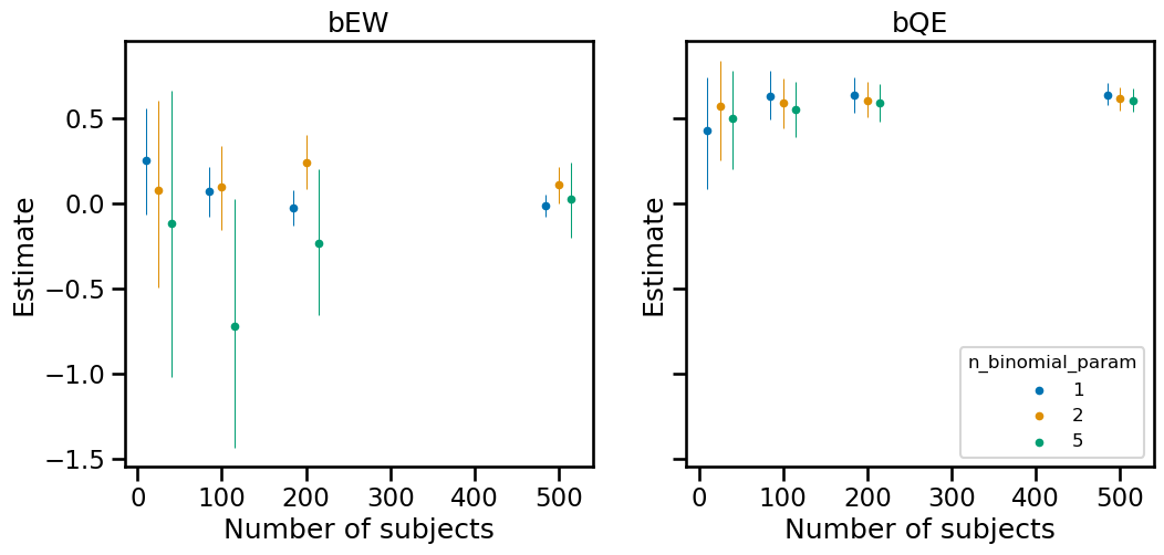
Results of experiments with generated data parameters
f, (ax0, ax1) = plt.subplots(1, 2, figsize=(12, 5), sharey=True)

def plot_mean_and_ci(coefficient, ax):
    x_shifts = [-15, 0, 15]
    n_binomial_param_list = [1, 2, 5]
    colors = cb_palette[0:3]
    for n_binom, x_shift, color in zip(n_binomial_param_list, x_shifts, colors):
        df = (
            df_summary.reset_index(names="coefficient")
            .query("coefficient==@coefficient")
            .query("n_binomial_param==@n_binom")
        )
        ax.scatter(df["num_subjects"]+x_shift, df["mean"], facecolors=None, edgecolor=color, s=2**4, label=n_binom)
        ax.vlines(x=df["num_subjects"]+x_shift, ymin=df["hdi_3%"], ymax=df["hdi_97%"], linewidth=0.75, color=color)
    ax.set_title(coefficient)
    ax.set(
        xlabel="Number of subjects",
        ylabel="Estimate"

    )
    if coefficient == "bQE":
        ax.legend(title='n_binomial_param', title_fontsize=12, fontsize=12, loc='lower right')

plot_mean_and_ci("bEW", ax0)
plot_mean_and_ci("bQE", ax1)
g = sns.relplot(
    data=df_summary.reset_index(names="coefficient"),
    x="num_subjects",
    y="sd",
    hue="n_binomial_param",
    hue_order = [1,2,5],
    col="coefficient",
    palette=cb_palette[0:3],
    kind='line'
)

g.set_titles(col_template="{col_name}")
g.set_axis_labels(x_var="Number of subjects", y_var="SD of coefficient")
plt.setp(g._legend.get_texts(), fontsize='12')
plt.setp(g._legend.get_title(), fontsize='12');
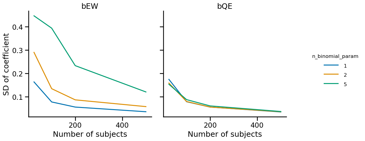
First, it makes sense that the variability of bQE is not affected by the binomial parameter since this coefficient is not dependent on the logit transformation. The variability of the bEW decreases with the number of subjects, as one might intuit. But I didn’t necessarily expect that a higher $n$ as a binomial parameter would lead to higher variability.
Summary and acknowledgements
My motivation for this post was understanding how to implement IV analysis with a binary outcome. I also ran an experiment to determine appropriate sample sizes. Some of the coding implementation was tricky for me initially. Thanks to the man himself for providing some help.
%load_ext watermark
%watermark -n -u -v -iv -w
The watermark extension is already loaded. To reload it, use:
  %reload_ext watermark
Last updated: Wed Jun 12 2024

Python implementation: CPython
Python version       : 3.12.3
IPython version      : 8.24.0

pymc      : 5.15.0
matplotlib: 3.8.4
scipy     : 1.13.0
seaborn   : 0.13.2
numpy     : 1.26.4
pandas    : 2.2.2
arviz     : 0.18.0
pytensor  : 2.20.0

Watermark: 2.4.3