Longitudinal Survey Designs
Notes for Chapter 4 of Causal Inference with Survey Data on LinkedIn Learning, given by Franz Buscha. I’m using this series of posts to take some notes.
import graphviz as gr
def draw_causal_graph(
    edge_list, node_props=None, edge_props=None, graph_direction="UD"
):
    """Utility to draw a causal (directed) graph
    Taken from: https://github.com/dustinstansbury/statistical-rethinking-2023/blob/a0f4f2d15a06b33355cf3065597dcb43ef829991/utils.py#L52-L66

    """
    g = gr.Digraph(graph_attr={"rankdir": graph_direction})

    edge_props = {} if edge_props is None else edge_props
    for e in edge_list:
        props = edge_props[e] if e in edge_props else {}
        g.edge(e[0], e[1], **props)

    if node_props is not None:
        for name, props in node_props.items():
            g.node(name=name, **props)
    return g
Surveys with longitudinal data
- A series of snapshots.
- Captures information from the same subjects across multiple points in time.
- Useful in understanding how relationships evolve and spotting trends.
Example: A training program
Cross-sectional
- snapshot
- static
- limited causality
- quick and cheap
Longitudinal
- time series
- dynamic (can follow someone’s productivity over time)
- better causality
- slow and expensive
Types of longitudinal data
- Panel survey
- Collect data on individuals, households, or companies over short time periods. Example: studies of demographic dynamics of families.
- Cohort survey
- Follow a group of people who share a common characteristic or experience within a defined survey.
- Repeated cross-section
- Collect data from different samples over time but from the same population.
Statistical Framework
- Key to working with time is the t subscript
- Time subscripts are manipulated by methods in different ways
Summary
- Allow for a deeper level of analysis, especially for cause-and-effect relationships
- Remember to consider challenges such as data attrition, time-carrying confounders, and complexity of such data
- They often provide a richer and more nuanced view of the world.
Regression models with time effects
- Adding time to a regression model can significantly improve causal inference
- Time flows in one direction
- Time trends and lagged values are common ways to include time
OLS with longitudinal data
- Work with time is the t subscript
- Static model makes no specific use of time from a methods perspective
- Time can be added to this model
Time manipulation: trends
- Time can be included as a variable (linear or otherwise)
- T is simply the survey time variable
- Many processes trend, so it makes sense to add time as a control
Time manipulation: lags
- Lags help explain how past values of X are related to present values of Y
- Help trace how past events affect today’s outcome
-
Termed finite distributed lag models of order N
- Model of order 2:
X1 and X2 are measured in the present. X3 is measured at three timepoints (present, lag of 1 and lag of 2.)
-
$\beta_3, \beta_4, \beta_5$ are independent; they are often summed to estimate a long-run effect of X on Y
-
Powerful model for estimating cause and effect of a variable
Summary
Advantages
- Capture dynamic effects
- Temporal causality
- Flexibility
Disadvantages
- Require lots of data
- Autocorrelation/multi-collinearity
- Reverse causality
Conclusion
- Using time in a regression can be a real game changer
- You can uncover short- and long-run effects, which cannot be done using static models
Fixed effects regression models
- A straightforward causal method that requires fewer theoretical assumptions.
- Has one major disadvantage - it’s terminal.
- Very frequently used with panel data.
Fixed effect: A DAG approach
- The focus is on variation over a data unit over time
- X2 and u are confounders
- X2 can be controlled for but not u
- Fixed effects removes both
draw_causal_graph(
    edge_list=[
        ("u", "X1_1"),
        ("u", "X1_2"),
        ("u", "X1_3"),
        ("u", "Y_1"),
        ("u", "Y_2"),
        ("u", "Y_3"),
        ("X2", "X1_1"),
        ("X2", "X1_2"),
        ("X2", "X1_3"),
        ("X2", "Y_1"),
        ("X2", "Y_2"),
        ("X2", "Y_3"),
        ("X1_1", "Y_1"),
        ("X1_2", "Y_2"),
        ("X1_3", "Y_3"),
        ("X1_1", "X1_2"),
        ("X1_2", "X1_3"),
    ],
    edge_props={
        ("u", "X1_1"): {"style": "dashed"},
        ("u", "X1_2"): {"style": "dashed"},
        ("u", "X1_3"): {"style": "dashed"},
        ("u", "Y1_1"): {"style": "dashed"},
        ("u", "Y1_2"): {"style": "dashed"},
        ("u", "Y1_3"): {"style": "dashed"},
    },
)

Implementing FE: LSDV
- Least Squares Dummy Variable approach (LSDV): include all panel units as dummy variables in a regression
Z is a large vector of dummy variables
- Estimate this using standard regression
- The many $\lambda$ terms control for time-invariant unobserved effects
- Method is disadvantaged if panel is large or limited hardware
Implementing FE: Within-transformation
-
The within-transformation subtracts the average panel unit value from each measured data point
-
The within-transformation subtracts the average panel unit value from each measured data point
- We’re removing data averages from each variable
- Variables that do not vary over time are removed from the model, including unobserved variables
Summary
Advantages
- Control for unobserved confounders
- More credible causal effects
Disadvantages
- Less efficient
- Cannot analyze time-invariant variables
- Time-varying confounders
Conclusion
- A powerful tool for longitudinal data structures
- Control for unobserved time-invariant confounders
- Always estimate FE models if you can, to see if the results differ
- Continue to think about time-varying confounders
Difference-in-difference estimation
- Older technique, relatively simple
- It can be done using only four numbers, which is often as good as advanced methods
- Compares the difference in outcomes before and after for two groups = the difference in the differences
- DiD is then the effect of the intervention
Basic DiD: Minimum Wages
- Famous study by Card and Kreuger, won Nobel Prize
- They were interested in the effect of minimum wages on employment
- Theory says it can be both good and bad
“Treated”:
- New Jersey: Feb 1992 = $4.25
- New Jersey: Nov 1992 = $5.05
- Difference = after - before
“Unreated control”:
- Pennsylvania: Feb 1992 = $4.25
- Pennsylvania: Nov 1992 = $4.25
Basic DiD: Minimum Wages (fast food restaurants)
| Average Employment FTE | New Jersey | Penn | Difference |
|---|---|---|---|
| Before | 20.44 | 23.33 | -2.89 |
| After | 21.03 | 21.17 | -0.14 |
| Difference | 0.59 | -2.16 | 2.76 |
To get the full effect of the minimum wage law on employment, in NJ, use the counterfactual: assume NJ would have been on the same trajectory as Penn. That’s why you take the difference of the differences ($ 0.59 - (-2.16) $).
Basic DiD: Visualization
Here is one example but this doesn’t apply to the NJ/Penn example.
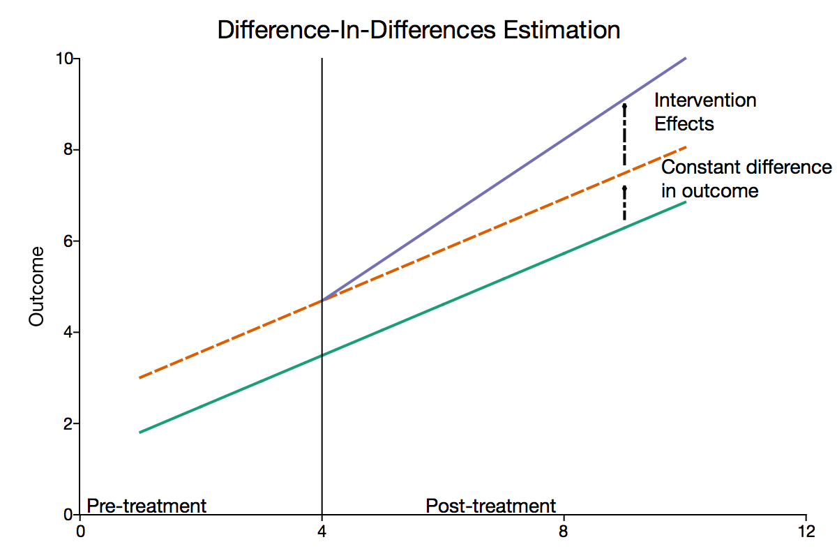
- Key assumption of DiD estimaton is the parallel trend assumption (if nothing had happened, NJ would follow same trend as Penn); represented by dashed line.
- The difference between the end of dashed line and labor supply in NJ is the DiD
Regression DiD
- Needed if there are additional confounders:
\(Y_{it} = \alpha + \beta_1 Treatment_i + \beta_2 Time_i + (\beta_3 Treatment_i \times Time_t) + \beta_4 X_{it} + \epsilon_{it}\) \(Treatment = \text{1 if treated, 0 if control}\) \(Time = \text{1 if post-period, 0 if pre-period}\) \(Treatment_i \times Time_t = \text{Interaction}\)
Assumptions
- Parallel trends
- No contamination
- Treatment cannot jump into control group and vice versa
Summary
Advantages
- Unobserved confounders
- Easy to apply
- Flexible (can be combined with other methods like matching techniques or standard regression techniques)
Disadvantages
- Requires assumptions to be met
- Can’t be used for single-case evaluations
Conclusions
- Popular evaluation strategy
- Need good quality data, at least two periods
- But it can offer compelling insights into the causal impact of policies and interventions, to help guide decision making
Synthetic control methods
- A new innovation in causal inference (last 15 years)
- Somewhat similar to DiD
- Creating a “synthetic control” that looks like the treated (using a weighted combination of potential control units)
- A great approach when no easy controls are available
Creating the synthetic control
- Synthetic control is the weighted sum of other potential control units
- Sum of weights, w, must equal to 1
Estimating the weights
- The weights minimize the difference between the treated unit and the control before the intervention
- Involves an optimization process
- Typically, it involves control variables that assist in matching the treated and synthetic units
Control variables
- Must be unaffected by the intervention/policy/treatment
- Typical control variables include economic or demographic indicators, and other pre-intervention attributes
- The quality of the synthetic control greatly depends on these variables
Evlauating the intervention
- The effect of the intervention is the difference between the treated unit and the synthetic control:
- Synthetic control estimates are tailored to recover the ATT.
Cross-Contamination is allowed
- This occurs when control units are affected by the intervention
- Allowed in scenarios where pure separation between treated and control isn’t possible, such as in geographic cases
Example: If CA impelements a new health policy, it’s likely neighboring states follow CA and implement some but not all policies. Neighboring control states are not clean. Example is Prop 99 for tobacco legislation.
Summary
Advantages
- Handling heterogeneity
- Complex interventions
Disdvantages
- Many pretreatment periods
- External validity
- Pre-intervention fit
Conclusion
- Synthetic control provides a sophisticated tool
- Especially useful for analysis of interventions that affect only one unit and cross-contamination exists
%load_ext watermark
%watermark -n -u -v -iv -w
Last updated: Tue May 28 2024

Python implementation: CPython
Python version       : 3.12.3
IPython version      : 8.24.0

graphviz: 0.20.3

Watermark: 2.4.3