When the Spider-Man meme is relevant to multilevel models

For a while, I’ve wondered about the different approches for multilevel modeling, also known as mixed effects modeling. My initial understanding is with a Bayesian perspective since I learned about it from Statistical Rethinking. But when hearing others talk about “fixed effects”, “varying effects”, “random effects”, and “mixed effects”, I had trouble connecting my own understanding of the concept to theirs. Even more perplexing, I wasn’t sure what the source(s) of the differences were:

• It it a frequentist vs. Bayesian thing?
• Is it a statistical package thing?
• Is it because there are five different definitions of “fixed and random effects”, infamously observed by Andrew Gelman and why he avoids using those terms?

I decided to take a deep dive to resolve my confusion, with much help from numerous sources. Please check out the Acknowledgments and references section!

In this post, I’ll be comparing an example of mixed effects modeling across statistical philosophies and across statistical languages. As a bonus, a meme awaits.

method	approach	language	package
1	frequentist	R	lme4
2	Bayesian	Python	pymc

Note that the default language in the code blocks is Python. A cell running R will have %%R designated at the top. A variable can be inputted (-i) or outputted (-o) on that same line if it is used between the two languages.

Special thanks to Patrick Robotham for providing a lot of feedback.

from aesara import tensor as at
import arviz as az
import matplotlib.pyplot as plt
import numpy as np
import os
import pandas as pd
import pymc as pm
import xarray as xr

%config InlineBackend.figure_format = 'retina'
az.style.use("arviz-darkgrid")
rng = np.random.default_rng(1234)
az.rcParams["stats.hdi_prob"] = 0.95 

def standardize(x):
    x = (x - np.mean(x)) / np.std(x)
    return x

# Enable running of R code
%load_ext rpy2.ipython

%%R
suppressMessages(library(tidyverse))
suppressMessages(library(lme4))
suppressMessages(library(arm))
suppressMessages(library(merTools))

Create synthetic cafe dataset

The dataset I am using is created from a scenario described in Statistical Rethinking.

Here are a few more details of the dataset from Dr. McElreath’s book:

Begin by defining the population of cafés that the robot might visit. This means we’ll define the average wait time in the morning and the afternoon, as well as the correlation between them. These numbers are sufficient to define the average properties of the cafés. Let’s define these properties, then we’ll sample cafés from them.

Nearly all Python code is taken from the Statistical Rethinking pymc repo with some minor alterations.

a = 3.5  # average morning wait time
b = -1.0  # average difference afternoon wait time
sigma_a = 1.0  # std dev in intercepts
sigma_b = 0.5  # std dev in slopes
rho = -0.7  # correlation between intercepts and slopes

Mu = [a, b]

sigmas = [sigma_a, sigma_b]
Rho = np.matrix([[1, rho], [rho, 1]])
Sigma = np.diag(sigmas) * Rho * np.diag(sigmas)  # covariance matrix

N_cafes = 20
vary_effects = np.random.multivariate_normal(mean=Mu, cov=Sigma, size=N_cafes)
a_cafe = vary_effects[:, 0]
b_cafe = vary_effects[:, 1]

Now simulate the observations.

N_visits = 10
afternoon = np.tile([0, 1], N_visits * N_cafes // 2)
cafe_id = np.repeat(np.arange(0, N_cafes), N_visits)

mu = a_cafe[cafe_id] + b_cafe[cafe_id] * afternoon
sigma = 0.5  # std dev within cafes

wait = np.random.normal(loc=mu, scale=sigma, size=N_visits * N_cafes)
df_cafes = pd.DataFrame(dict(cafe=cafe_id, afternoon=afternoon, wait=wait))

To get a sense of the data structure we just created, let’s take a look at the first and last 5 rows.

df_cafes.head()

	cafe	afternoon	wait
0	0	0	2.724888
1	0	1	1.951626
2	0	0	2.488389
3	0	1	1.188077
4	0	0	2.026425

df_cafes.tail()

	cafe	afternoon	wait
195	19	1	3.394933
196	19	0	4.544430
197	19	1	2.719524
198	19	0	3.379111
199	19	1	2.459750

Note that this dataset is balanced, meaning that each group (cafe) has the same number of observations. Mixed effects / multilevel models shine with unbalanced data where it can leverage partial pooling.

Visualize data

Let’s plot the raw data and see how the effect of afternoon influences wait time. Instead of plotting in order of the arbitrarily named cafes (0 to 19), I’ll show in order of increasing average morning wait time so that we can appreciate the variability across the dataset.

df_cafes.head()

	cafe	afternoon	wait
0	0	0	2.644592
1	0	1	2.126485
2	0	0	2.596465
3	0	1	2.250297
4	0	0	3.310709

%%R -i df_cafes

# credit to TJ Mahr for a template of this code
xlab <- "Afternoon"
ylab <- "Wait time"
titlelab <- "Wait times for each cafe (ordered by increasing average time)"

# order by increasing average morning wait time (intercept only)
cafe_ordered_by_avgwaittime <- df_cafes %>%
              filter(afternoon==0) %>%
              group_by(cafe) %>%
              summarize(mean = mean(wait)) %>%
              arrange(mean)

# Turn the gear column from a numeric in a factor with a certain order
df_cafes$cafe <- factor(df_cafes$cafe, levels=cafe_ordered_by_avgwaittime$cafe)

ggplot(df_cafes) + 
  aes(x = afternoon, y = wait) + 
  geom_boxplot(aes(fill=factor(afternoon))) +
  stat_summary(fun.y="mean", geom="line") +
  facet_wrap("cafe") +
  labs(x = xlab, y = ylab, title=titlelab)

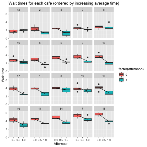
One pattern is that as we increase morning wait time (e.g. the intercept) the difference in wait time in the afternoon (the slope) gets bigger. In other words, when we simulated this dataset, we included a co-variance structure between the intercept and slope. When we develop an inferential model with this data, we want to be able to reveal this co-variance.

Definitions of mixed effects modeling

Equation set 1: both fixed and random effects terms in linear model

Galecki and Burzykowski, Wikipedia, and this page from UCLA all describe a linear mixed model with an equation similar to equation 1 below.

I rely heavily on the UCLA page since it is the one that helped me the most. In fact, if you don’t care about how it connects to the Bayesian approach, stop reading this and check that out instead!

In contrast to the Bayesian set of equations, the fixed effects and random effects are in the same equation here.

\[\textbf{y} = \textbf{X} \boldsymbol{\beta} + \textbf{Z} \textbf{u} + \boldsymbol{\epsilon} \tag{1}\]

The left side of the equation $\textbf{y}$ represents all of our observations (or the wait time in the cafe example). The $\boldsymbol{\beta}$ in the first term of the equation represents a vector of coefficients across the population of cafes. These are the fixed effects. The $\textbf{u}$ in the second term of equation 1 represents a matrix of coefficients for each individual cafe. These are the random effects. Both $\textbf{X}$ and $\textbf{Z}$ are the design matrix of covariates. Finally, there’s a residual error term $\boldsymbol{\epsilon}$.

When relating this equation all back to the cafe dataset we just created, I needed to dig deeper to how terms represented an individual observation versus the group (cafe) level. Doing a dimensional analysis helped.

Equation 1 variable	Dimensions	Effects type	Comment
$\textbf{y}$	200 x 1	n/a	This vector represents the wait time for all 200 observations. I’ll refer to this as $w_i$ later in equation 2.
$\textbf{X}$	200 x 2	associated with fixed	The first column of each observation is 1 since it is multiplied by the intercept term. The second column is $A$, which will be 0 or 1 for afternoon.
$\boldsymbol{\beta}$	2 x 1	fixed	The two elements in the $\boldsymbol{\beta}$ (bold font beta) are what I’ll refer to as the intercept $\alpha$ and the slope $\beta$ (unbolded beta) across all cafes in equation 2.
$\textbf{Z}$	200 x (2x20)	associated with random	The first 20 columns representing intercepts for each cafe and the second 20 for the covariate (afternoon). See visual below.
$\textbf{u}$	(2x20) x 1	random	$\textbf{u}$ holds each of the 20 cafes’ intercept $a_\text{cafe}$ and slope $b_\text{cafe}$. There’s an implied correlation structure between them.
$\boldsymbol{\epsilon}$	200 x 1	n/a	Normally distributed residual error.

To better understand what $\textbf{Z}$ looks like we can create an alternate representation of df_cafes. Each row of the matrix $\textbf{Z}$ is for an individual observation. The first 20 columns of a row are the 20 intercepts of a cafe (column 1 is cafe 1, column 2 is cafe 2, etc.) All of the first 20 columns will contain a 0 except for the column that represents the cafe that observation is associated with which will be a 1. The next 20 columns (columns 21-40) will represent afternoon. All of this second group of columns will be 0 except for the column that represents the cafe that observation is associated with and if the observation is associated with an afternon observation.

To be clear, the structure of df_cafes, where each row is an observation with the cafe, afternoon status, and wait time, is already in a form to be understood by the lmer and pymc packages. What I’m showing below is to help understand what the matrix $\textbf{Z}$ looks like in the above equations.

Z = np.zeros((200, 40))
for i in df_cafes.index:
    cafe = df_cafes.loc[i, 'cafe']
    afternoon = df_cafes.loc[i, 'afternoon']
    Z[i, cafe] = 1
    Z[i, 20+cafe] = afternoon

We can take a look at the first 12 rows of Z. The first 10 are for the first cafe and observations alternate morning and afternoon, hence what’s displayed in column 20. I included the first two rows of the second cafe to show how the 1 moves over a row after the first 10 rows. I’ll use pandas to better display the values.

pd.set_option('display.max_columns', 40)
(
    pd.DataFrame(Z[0:12, :])
    .astype(int)
    .style
    .highlight_max(axis=1, props='color:navy; background-color:yellow;')
    .highlight_min(axis=1, props='color:white; background-color:#3E0B51;')
)

	0	1	2	3	4	5	6	7	8	9	10	11	12	13	14	15	16	17	18	19	20	21	22	23	24	25	26	27	28	29	30	31	32	33	34	35	36	37	38	39
0	1	0	0	0	0	0	0	0	0	0	0	0	0	0	0	0	0	0	0	0	0	0	0	0	0	0	0	0	0	0	0	0	0	0	0	0	0	0	0	0
1	1	0	0	0	0	0	0	0	0	0	0	0	0	0	0	0	0	0	0	0	1	0	0	0	0	0	0	0	0	0	0	0	0	0	0	0	0	0	0	0
2	1	0	0	0	0	0	0	0	0	0	0	0	0	0	0	0	0	0	0	0	0	0	0	0	0	0	0	0	0	0	0	0	0	0	0	0	0	0	0	0
3	1	0	0	0	0	0	0	0	0	0	0	0	0	0	0	0	0	0	0	0	1	0	0	0	0	0	0	0	0	0	0	0	0	0	0	0	0	0	0	0
4	1	0	0	0	0	0	0	0	0	0	0	0	0	0	0	0	0	0	0	0	0	0	0	0	0	0	0	0	0	0	0	0	0	0	0	0	0	0	0	0
5	1	0	0	0	0	0	0	0	0	0	0	0	0	0	0	0	0	0	0	0	1	0	0	0	0	0	0	0	0	0	0	0	0	0	0	0	0	0	0	0
6	1	0	0	0	0	0	0	0	0	0	0	0	0	0	0	0	0	0	0	0	0	0	0	0	0	0	0	0	0	0	0	0	0	0	0	0	0	0	0	0
7	1	0	0	0	0	0	0	0	0	0	0	0	0	0	0	0	0	0	0	0	1	0	0	0	0	0	0	0	0	0	0	0	0	0	0	0	0	0	0	0
8	1	0	0	0	0	0	0	0	0	0	0	0	0	0	0	0	0	0	0	0	0	0	0	0	0	0	0	0	0	0	0	0	0	0	0	0	0	0	0	0
9	1	0	0	0	0	0	0	0	0	0	0	0	0	0	0	0	0	0	0	0	1	0	0	0	0	0	0	0	0	0	0	0	0	0	0	0	0	0	0	0
10	0	1	0	0	0	0	0	0	0	0	0	0	0	0	0	0	0	0	0	0	0	0	0	0	0	0	0	0	0	0	0	0	0	0	0	0	0	0	0	0
11	0	1	0	0	0	0	0	0	0	0	0	0	0	0	0	0	0	0	0	0	0	1	0	0	0	0	0	0	0	0	0	0	0	0	0	0	0	0	0	0

We can visualize all of $\textbf{Z}$ here.

plt.imshow(Z, aspect='auto')
plt.text(10, 220, s='intercept (cafe)', ha='center', fontsize=14)
plt.text(30, 220, s='covariate (afternoon)', ha='center', fontsize=14)
plt.ylabel('observations')
plt.title('Visual representation of Z')

Text(0.5, 1.0, 'Visual representation of Z')

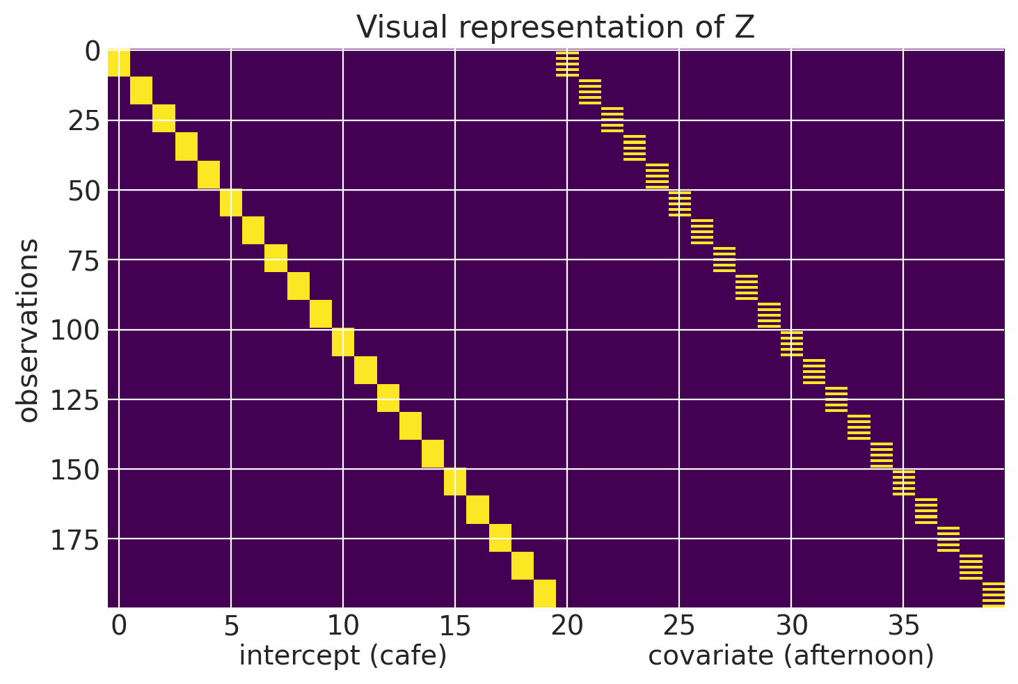
The vector in $\textbf{u}$ is really where the mixed effects model takes advantage of the covariance structure of the data. In our dataset, the first 20 elements of the vector represent the random intercepts of the cafes and the next 20 are the random slopes. A cafe’s random effects can be thought of as an offset from the populations (the fixed effects). Accordingly, a random effect will be multivariate normally distributed, with mean 0 and a co-variance matrix S.

\[\textbf{u} \sim \text{Normal}(0, \textbf{S}) \tag{2}\]

Remember that the $\textbf{u}$ is a (2x20) x 1 matrix, where each cafe’s intercept $a_\text{cafe}$ and slope $b_\text{cafe}$ are contained. Therefore, we can also write this as.

\[\textbf{u} = \begin{bmatrix} a_{\text{cafe}} \\ b_{\text{cafe}} \end{bmatrix} \sim \text{MVNormal} \left( \begin{bmatrix} 0 \\ 0 \end{bmatrix} , \textbf{S} \right) \tag{3}\]

In other words, in Equation 1, both the random intercept and random slope are both expected to lie at 0. With regards to $\textbf{S}$, my prior post talked about covariance matrixes so I won’t elaborate here. The key conceptual point of relevance in this problem is that the covariance matrix $\textbf{S}$ can reflect the correlation ($\rho$) that the intercept (average morning wait time) and slope (difference between morning and afternoon wait time).

\[\textbf{S} = \begin{pmatrix} \sigma_{\alpha}^2 & \rho\sigma_{\alpha}\sigma_{\beta} \\ \rho\sigma_{\alpha}\sigma_{\beta} & \sigma_{\beta}^2 \end{pmatrix} \tag{4}\]

We know there is a correlation because (a) we generated the data that way and (b) we can directly observe this when we visualized the data.

Finally, the role of $\boldsymbol{\epsilon}$ is to capture any residual variance. Between observations, it is assumed to be homogenous and independent.

Non-linear algebra form

Equation 1 is written concisely in linear algebra form. However, since our dataset is relatively simple (only one predictor variable), equation 1 can be written in an expanded, alternative form as equation 2. This might make it easier to understand (at least it did for me). The notation will start to get hairy with subscripts and so I will explicitly rename some variables for this explanation. It will also better match with the Bayesian set of equations described in the McElreath text. Equation 2 is written at the level of a single observation $i$. I’ll repeat Equation 1 here so it’s easier to see the conversion.

\[\textbf{y} = \textbf{X} \boldsymbol{\beta} + \textbf{Z} \textbf{u} + \boldsymbol{\epsilon} \tag{5}\] \[W_i = (\alpha + \beta \times A_i) + (a_{\text{cafe}[i]} + b_{\text{cafe}[i]} \times A_i) + \epsilon_i \tag{6}\]

Let’s start off with the left side where we can see that $\textbf{y}$ will now be $W_i$ for wait time. On the right side, I have segmented the fixed and random effects with parentheses. For both, I’ve deconstructed the linear algebra expression form to a simpler form. After re-arrangement, we can obtain the following form in equation 3.

\[W_i = (\alpha + a_{\text{cafe}[i]}) + (\beta + b_{\text{cafe}[i]}) \times A_i + \epsilon_{\text{cafe}} \tag{7}\]

Here, we can better appreciate how a cafe’s random effects intercept can be thought of as an offset from the population intercept. The same logic of an offset can be applied to its slope. We will come back to equation 3 after covering Equation set 2, the Bayesian approach.

Equation set 2: fixed effects as an adaptive prior, varying effects in the linear model

The following equations are taken from Chapter 14 in Statistical Rethinking. These set of equations look like a beast, but to be honest, they’re more intuitive to me, probably because I learned this approach initially. I’ll state the equations before comparing them directly with Equation set 1 but you may already start seeing the relationship. Essentially what is going on is a re-writing of the above equations in a Bayesian way such that the fixed effects can act as an adaptive prior.

\(W_i \sim \text{Normal}(\mu_i, \sigma) \tag{8}\) \(\mu_i = \alpha_{\text{cafe}[i]} + \beta_{\text{cafe}[i]} \times A_{i} \tag{9}\) \(\sigma \sim \text{Exp}(1) \tag{10}\)

Equation 8 is stating how wait time is normally distributed around $\mu$ and $\sigma$. By making $w_i$ stochastic instead of deterministic (using a ~ instead of =), the $\sigma$ replaces $\epsilon_i$. In equation 10, the prior for $\sigma$ is exponentially distributed and paramaterized with 1. The expected value parameter $\mu$ comes from the linear model in equation 9. You can start to see the similarities with equation 7 above.

\[\begin{bmatrix}\alpha_{\text{cafe}} \\ \beta_{\text{cafe}} \end{bmatrix} \sim \text{MVNormal} \left( \begin{bmatrix}{\alpha} \\ {\beta} \end{bmatrix} , \textbf{S} \right) \tag{11}\]

The $\alpha_{\text{cafe}}$ and $\beta_{\text{cafe}}$ terms come from sampling of a multivariate normal distribution as shown in equation 11. Note the very subtle difference in placement of the subscript cafe when compared to equation 6 and 7. This is an important point I’ll discuss later. On the right side, the two-dimensional normal distribution’s expected values are $\alpha$ and $\beta$. The rest of the equations shown below are our priors for each parameter we’re trying to estimate.

\[\alpha \sim \text{Normal}(5, 2) \tag{13}\] \[\beta \sim \text{Normal}(-1, 0.5) \tag{14}\] \[\textbf{S} = \begin{pmatrix} \sigma_{\alpha}^2 & \rho\sigma_{\alpha}\sigma_{\beta} \\ \rho\sigma_{\alpha}\sigma_{\beta} & \sigma_{\beta}^2 \end{pmatrix} = \begin{pmatrix} \sigma_{\alpha} & 0 \\ 0 & \sigma_{\beta} \end{pmatrix} \textbf{R} \begin{pmatrix} \sigma_{\alpha} & 0 \\ 0 & \sigma_{\beta} \end{pmatrix} \tag{12}\]

\(\sigma, \sigma_{\alpha}, \sigma_{\beta} \sim \text{Exp}(1) \tag{15}\) \(\textbf{R} \sim \text{LKJCorr}(2) \tag{16}\)

Comparison of equation sets

To recap, the first equation set has an explicit fixed effects term and varying effects term in the linear model. In the second equation, the linear model is already “mixed”. It contains both the fixed and varying effects terms implicitly. The fixed effects estimates can be seen in equation 5.

I think you can think of these $\alpha_{\text{cafe}}$ and $\beta_{\text{cafe}}$ terms as already incorporating the information from the fixed and random effects simultaneously.

Now that we have the dataset, we can run the two models, one with lmer and one with pymc. Here are the equations that these packages run.

Running equation set 1 with lmer (frequentist)

The lmer and by extension (brms) syntax was initially confusing to me.

lmer(wait ~ 1 + afternoon + (1 + afternoon | cafe), df_cafes)

The 1 corresponds to inclusion of the intercept term. A 0 would exclude it. The 1 + wait corresponds to the “fixed effects” portion of the model ($\alpha + \beta \times A_i$) while the (1 + wait | cafe) is the “varying effects” ($a_{\text{cafe}} + b_{\text{cafe}} \times A_i$).

%%R -i df_cafes -o m -o df_fe_estimates -o df_fe_ci -o df_fe_summary

# m df_fe_summary
m <- lmer(wait ~ 1 + afternoon + (1 + afternoon | cafe), df_cafes)
arm::display(m)

# get fixed effects coefficients
df_fe_estimates <- data.frame(summary(m)$coefficients)
# get fixed effects coefficient CIs
df_fe_ci <- data.frame(confint(m))

df_fe_summary <- merge(
    df_fe_estimates,
    df_fe_ci[c('(Intercept)', 'afternoon'), ],
    by.x=0,
    by.y=0
)
rownames(df_fe_summary) <- df_fe_summary[, 1]

lmer(formula = wait ~ 1 + afternoon + (1 + afternoon | cafe), 
    data = df_cafes)
            coef.est coef.se
(Intercept)  3.64     0.23  
afternoon   -1.04     0.11  

Error terms:
 Groups   Name        Std.Dev. Corr  
 cafe     (Intercept) 0.99           
          afternoon   0.39     -0.74 
 Residual             0.48           
---
number of obs: 200, groups: cafe, 20
AIC = 369.9, DIC = 349.2
deviance = 353.5 


R[write to console]: Computing profile confidence intervals ...

Can we get the partial pooling results from the lmer output and see how it compares with the unpooled estimates? Let’s export it for use later.

%%R -i m -o df_partial_pooling -o random_sims

# Make a dataframe with the fitted effects
df_partial_pooling <- coef(m)[["cafe"]] %>% 
  rownames_to_column("cafe") %>% 
  as_tibble() %>% 
  rename(Intercept = `(Intercept)`, Slope_Days = afternoon) %>% 
  add_column(Model = "Partial pooling")

# estimate confidence interval
random_sims <- REsim(m, n.sims = 1000)
#plotREsim(random_sims)

random_sims

	groupFctr	groupID	term	mean	median	sd
1	cafe	0	(Intercept)	-1.277651	-1.283341	0.379761
2	cafe	1	(Intercept)	0.164935	0.162715	0.420411
3	cafe	2	(Intercept)	-1.047076	-1.043646	0.387153
4	cafe	3	(Intercept)	0.474320	0.500552	0.400053
5	cafe	4	(Intercept)	-1.473647	-1.468940	0.394707
6	cafe	5	(Intercept)	0.086072	0.082010	0.408971
7	cafe	6	(Intercept)	-0.640217	-0.628944	0.412642
8	cafe	7	(Intercept)	1.507154	1.516430	0.391119
9	cafe	8	(Intercept)	-0.657831	-0.659448	0.394984
10	cafe	9	(Intercept)	0.332758	0.331037	0.388295
11	cafe	10	(Intercept)	-1.018611	-1.025387	0.389930
12	cafe	11	(Intercept)	0.925071	0.913997	0.397095
13	cafe	12	(Intercept)	-1.407149	-1.403259	0.384820
14	cafe	13	(Intercept)	-0.412975	-0.414958	0.412863
15	cafe	14	(Intercept)	1.346380	1.343109	0.403694
16	cafe	15	(Intercept)	0.336807	0.346523	0.390567
17	cafe	16	(Intercept)	0.747439	0.735906	0.413094
18	cafe	17	(Intercept)	-0.046579	-0.035018	0.396795
19	cafe	18	(Intercept)	1.659019	1.646634	0.393909
20	cafe	19	(Intercept)	0.323375	0.327348	0.392401
21	cafe	0	afternoon	0.498557	0.501401	0.182594
22	cafe	1	afternoon	-0.336036	-0.337360	0.193462
23	cafe	2	afternoon	0.395379	0.391621	0.189140
24	cafe	3	afternoon	0.296956	0.293144	0.191710
25	cafe	4	afternoon	0.059611	0.055121	0.189680
26	cafe	5	afternoon	-0.033068	-0.036143	0.194723
27	cafe	6	afternoon	0.236107	0.237904	0.192575
28	cafe	7	afternoon	-0.473485	-0.479199	0.185549
29	cafe	8	afternoon	0.408039	0.411507	0.194145
30	cafe	9	afternoon	-0.402131	-0.393931	0.186868
31	cafe	10	afternoon	0.316072	0.309198	0.189218
32	cafe	11	afternoon	-0.335749	-0.340427	0.186644
33	cafe	12	afternoon	0.521558	0.519243	0.184606
34	cafe	13	afternoon	-0.006800	-0.014344	0.199548
35	cafe	14	afternoon	-0.277165	-0.281127	0.188748
36	cafe	15	afternoon	-0.234501	-0.235683	0.192804
37	cafe	16	afternoon	-0.182673	-0.185997	0.194017
38	cafe	17	afternoon	-0.017126	-0.023784	0.187302
39	cafe	18	afternoon	-0.364424	-0.364049	0.187532
40	cafe	19	afternoon	-0.028883	-0.032691	0.185824

OK, now let’s try the Bayesian approach and compare answers.

Running equation set 2 with pymc (Bayesian)

n_cafes = df_cafes['cafe'].nunique()
cafe_idx = pd.Categorical(df_cafes["cafe"]).codes

with pm.Model() as m14_1:
    # can't specify a separate sigma_a and sigma_b for sd_dist but they're equivalent here
    chol, Rho_, sigma_cafe = pm.LKJCholeskyCov(
        "chol_cov", n=2, eta=2, sd_dist=pm.Exponential.dist(1.0), compute_corr=True
    )
    
    a_bar = pm.Normal("a_bar", mu=5, sigma=2.0)  # prior for average intercept
    b_bar = pm.Normal("b_bar", mu=-1, sigma=0.5)  # prior for average slope

    
    ab_subject = pm.MvNormal(
        "ab_subject", mu=at.stack([a_bar, b_bar]), chol=chol, shape=(n_cafes, 2)
    )  # population of varying effects
    # shape needs to be (n_cafes, 2) because we're getting back both a and b for each cafe

    mu = ab_subject[cafe_idx, 0] + ab_subject[cafe_idx, 1] * df_cafes["afternoon"].values  # linear model
    sigma_within = pm.Exponential("sigma_within", 1.0)  # prior stddev within cafes (in the top line)

    wait = pm.Normal("wait", mu=mu, sigma=sigma_within, observed=df_cafes["wait"].values)  # likelihood

    idata_m14_1 = pm.sample(1000, target_accept=0.9)

Auto-assigning NUTS sampler...
Initializing NUTS using jitter+adapt_diag...
Multiprocess sampling (4 chains in 4 jobs)
NUTS: [chol_cov, a_bar, b_bar, ab_subject, sigma_within]

100.00% [8000/8000 02:03<00:00 Sampling 4 chains, 1 divergences]

Sampling 4 chains for 1_000 tune and 1_000 draw iterations (4_000 + 4_000 draws total) took 140 seconds.
There was 1 divergence after tuning. Increase `target_accept` or reparameterize.

# take a glimpse at the head and tail of the summary table
pd.concat(
    [
        az.summary(idata_m14_1).head(10),
        az.summary(idata_m14_1).tail(10)
    ]
)

/Users/blacar/opt/anaconda3/envs/pymc_env2/lib/python3.10/site-packages/arviz/stats/diagnostics.py:586: RuntimeWarning: invalid value encountered in double_scalars
  (between_chain_variance / within_chain_variance + num_samples - 1) / (num_samples)
/Users/blacar/opt/anaconda3/envs/pymc_env2/lib/python3.10/site-packages/arviz/stats/diagnostics.py:586: RuntimeWarning: invalid value encountered in double_scalars
  (between_chain_variance / within_chain_variance + num_samples - 1) / (num_samples)

	mean	sd	hdi_2.5%	hdi_97.5%	mcse_mean	mcse_sd	ess_bulk	ess_tail	r_hat
a_bar	3.654	0.223	3.203	4.074	0.003	0.002	4802.0	3140.0	1.0
b_bar	-1.049	0.109	-1.265	-0.844	0.002	0.001	3446.0	3200.0	1.0
ab_subject[0, 0]	2.380	0.200	1.996	2.785	0.003	0.002	4271.0	2783.0	1.0
ab_subject[0, 1]	-0.587	0.245	-1.071	-0.119	0.004	0.003	3077.0	2833.0	1.0
ab_subject[1, 0]	3.820	0.199	3.442	4.220	0.003	0.002	3988.0	3167.0	1.0
ab_subject[1, 1]	-1.402	0.248	-1.897	-0.945	0.004	0.003	3165.0	3182.0	1.0
ab_subject[2, 0]	2.606	0.199	2.210	2.988	0.003	0.002	4702.0	3450.0	1.0
ab_subject[2, 1]	-0.681	0.240	-1.156	-0.218	0.004	0.003	3696.0	3014.0	1.0
ab_subject[3, 0]	4.120	0.203	3.739	4.532	0.003	0.002	3475.0	2800.0	1.0
ab_subject[3, 1]	-0.707	0.266	-1.213	-0.184	0.005	0.004	2482.0	2921.0	1.0
chol_cov[0]	0.988	0.163	0.710	1.328	0.002	0.002	5207.0	3263.0	1.0
chol_cov[1]	-0.226	0.105	-0.442	-0.033	0.002	0.001	2769.0	3178.0	1.0
chol_cov[2]	0.299	0.093	0.120	0.481	0.002	0.002	1379.0	1308.0	1.0
sigma_within	0.482	0.027	0.431	0.534	0.000	0.000	3773.0	2542.0	1.0
chol_cov_corr[0, 0]	1.000	0.000	1.000	1.000	0.000	0.000	4000.0	4000.0	NaN
chol_cov_corr[0, 1]	-0.579	0.192	-0.898	-0.196	0.003	0.002	3196.0	2983.0	1.0
chol_cov_corr[1, 0]	-0.579	0.192	-0.898	-0.196	0.003	0.002	3196.0	2983.0	1.0
chol_cov_corr[1, 1]	1.000	0.000	1.000	1.000	0.000	0.000	4087.0	4000.0	1.0
chol_cov_stds[0]	0.988	0.163	0.710	1.328	0.002	0.002	5207.0	3263.0	1.0
chol_cov_stds[1]	0.386	0.107	0.182	0.605	0.003	0.002	1541.0	1201.0	1.0

Comparison of lmer and pymc outputs

While pymc returns posterior estimates for each parameter, including $\rho$, for this post, we are interested in comparing the output comparable to the “fixed effects” and “varying effects” from lmer. Having the equations above can help us piece together the relevant bits of information. The fixed intercept and slope are easy because we’ve used the same characters $\alpha$ and $\beta$ in equation set 2 as we did in Equation set 1.

However, when identifying the “varying effects”, we’ll have to do some arithmetic with the pymc output. In contrast with the lmer output, the pymc outputs have the estimate for each cafe with “baked in” varying effects. In other words, the “offset” that we see in equation 7 ($a_{\text{cafe}[i]}$ and $b_{\text{cafe}[i]}$)

\[W_i = (\alpha + a_{\text{cafe}[i]}) + (\beta + b_{\text{cafe}[i]}) \times A_i + \epsilon_{\text{cafe}} \tag{7}\] \[\mu_i = \alpha_{\text{cafe}[i]} + \beta_{\text{cafe}[i]} \times A_{i} \tag{9}\]

are already embedded in ($\alpha_{\text{cafe}[i]}$ and $\beta_{\text{cafe}[i]}$) in equation 9. We’ll have to therefore subtract out the fixed effecs in the pymc output before we can compare with the lmer output. First, let’s get fixed effects from pymc.

df_summary_int_and_slope = az.summary(idata_m14_1, var_names=['a_bar', 'b_bar'])
df_summary_int_and_slope

	mean	sd	hdi_2.5%	hdi_97.5%	mcse_mean	mcse_sd	ess_bulk	ess_tail	r_hat
a_bar	3.654	0.223	3.203	4.074	0.003	0.002	4802.0	3140.0	1.0
b_bar	-1.049	0.109	-1.265	-0.844	0.002	0.001	3446.0	3200.0	1.0

These estimates and uncertainties compare well with the fixed estimates lmer.

f, (ax0, ax1) = plt.subplots(1, 2, figsize=(12,4))
# value to generate data
# a, average morning wait time was defined above
ax0.vlines(x=a, ymin=0.8, ymax=1.2, linestyle='dashed', color='red')
ax1.vlines(x=b, ymin=0.8, ymax=1.2, linestyle='dashed', color='red', label='simulated value')

# pymc fixed effects value
ax0.scatter(df_summary_int_and_slope.loc['a_bar', 'mean'], 1.1, color='navy')
ax0.hlines(xmin=df_summary_int_and_slope.loc['a_bar', 'hdi_2.5%'], xmax=df_summary_int_and_slope.loc['a_bar', 'hdi_97.5%'], y=1.1, color='navy')
ax1.scatter(df_summary_int_and_slope.loc['b_bar', 'mean'], 1.1, color='navy')
ax1.hlines(xmin=df_summary_int_and_slope.loc['b_bar', 'hdi_2.5%'], xmax=df_summary_int_and_slope.loc['b_bar', 'hdi_97.5%'], y=1.1, color='navy', label='pymc estimate')

# lmer fixed effects estimate
ax0.scatter(df_fe_summary.loc['(Intercept)', 'Estimate'], 0.9, color='darkgreen')
ax0.hlines(xmin=df_fe_summary.loc['(Intercept)', 'X2.5..'], xmax=df_fe_summary.loc['(Intercept)', 'X97.5..'], y=0.9, color='darkgreen')
ax1.scatter(df_fe_summary.loc['afternoon', 'Estimate'], 0.9, color='darkgreen')
ax1.hlines(xmin=df_fe_summary.loc['afternoon', 'X2.5..'], xmax=df_fe_summary.loc['afternoon', 'X97.5..'], y=0.9, color='darkgreen', label='lmer estimate')

# plot formatting
f.suptitle('Fixed effect estimates')
ax0.set_yticks([0.9, 1.1])
ax0.set_yticklabels(['lmer', 'pymc'])

ax1.set_yticks([0.9, 1.1])
ax1.set_yticklabels(['', ''])

ax0.set(xlabel='intercept')
ax1.set(xlabel='slope')
ax1.legend(fontsize=10)
plt.tight_layout()

/var/folders/tw/b9j0wcdj6_9cyljwt364lx7c0000gn/T/ipykernel_5516/1253574855.py:30: UserWarning: This figure was using constrained_layout, but that is incompatible with subplots_adjust and/or tight_layout; disabling constrained_layout.
  plt.tight_layout()

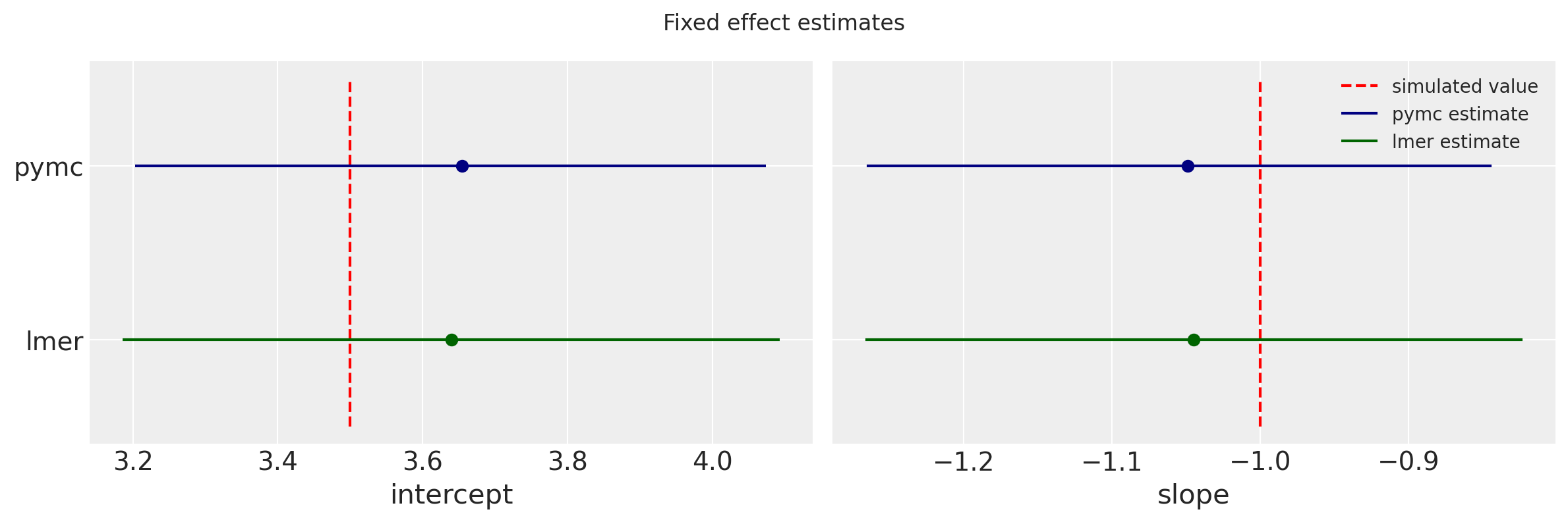
As promised, here is the meme that rewards you for paying attention this far!

Now to get the varying effects from pymc output, we’ll take each sample’s intercept and slope and subtract the fixed estimate.

# Convert to pandas dataframe and take a glimpse at the first few rows
idata_m14_1_df = idata_m14_1.to_dataframe()
idata_m14_1_df.head()

	chain	draw	(posterior, a_bar)	(posterior, b_bar)	(posterior, ab_subject[0,0], 0, 0)	(posterior, ab_subject[0,1], 0, 1)	(posterior, ab_subject[1,0], 1, 0)	(posterior, ab_subject[1,1], 1, 1)	(posterior, ab_subject[10,0], 10, 0)	(posterior, ab_subject[10,1], 10, 1)	(posterior, ab_subject[11,0], 11, 0)	(posterior, ab_subject[11,1], 11, 1)	(posterior, ab_subject[12,0], 12, 0)	(posterior, ab_subject[12,1], 12, 1)	(posterior, ab_subject[13,0], 13, 0)	(posterior, ab_subject[13,1], 13, 1)	(posterior, ab_subject[14,0], 14, 0)	(posterior, ab_subject[14,1], 14, 1)	(posterior, ab_subject[15,0], 15, 0)	(posterior, ab_subject[15,1], 15, 1)	...	(log_likelihood, wait[97], 97)	(log_likelihood, wait[98], 98)	(log_likelihood, wait[99], 99)	(log_likelihood, wait[9], 9)	(sample_stats, tree_depth)	(sample_stats, max_energy_error)	(sample_stats, process_time_diff)	(sample_stats, perf_counter_diff)	(sample_stats, energy)	(sample_stats, step_size_bar)	(sample_stats, diverging)	(sample_stats, energy_error)	(sample_stats, lp)	(sample_stats, acceptance_rate)	(sample_stats, n_steps)	(sample_stats, largest_eigval)	(sample_stats, smallest_eigval)	(sample_stats, index_in_trajectory)	(sample_stats, step_size)	(sample_stats, perf_counter_start)
0	0	0	3.397744	-0.993140	2.353823	-0.712216	3.936642	-1.328451	2.497521	-0.990675	4.589760	-1.271864	2.272038	-0.780358	3.400074	-1.307487	4.660517	-0.920542	3.967868	-1.339014	...	-0.592594	-0.280869	-1.783441	-0.404212	5	-0.452539	0.234946	0.067260	194.679539	0.246795	False	-0.226605	-167.432037	0.975607	31.0	NaN	NaN	-17	0.284311	192.355518
1	0	1	3.227032	-1.105823	2.486742	-0.657790	3.890044	-1.788579	2.894867	-0.741011	4.346072	-1.048541	2.446301	-0.678041	3.564795	-1.520221	5.013627	-1.128684	3.793134	-1.084814	...	-0.581570	-0.708670	-1.709776	-0.741664	4	0.498338	0.123327	0.033713	196.867266	0.246795	False	0.273832	-177.694232	0.809115	15.0	NaN	NaN	-8	0.284311	192.423125
2	0	2	3.393307	-0.926431	2.348434	-0.604619	3.905778	-1.355137	2.712834	-1.124770	4.409195	-1.291088	2.324233	-0.754508	3.586107	-1.562165	5.050191	-1.556993	4.122478	-1.718417	...	-0.452885	-0.109849	-2.293094	-0.559207	5	-0.382814	0.236803	0.063232	207.926089	0.246795	False	-0.347905	-176.112370	0.968229	31.0	NaN	NaN	6	0.284311	192.457135
3	0	3	3.750943	-1.109148	2.613325	-0.667234	3.682009	-1.293790	2.558511	-0.362557	4.548968	-1.266139	2.264383	-0.445725	3.102086	-0.903726	4.589499	-0.409875	4.063760	-1.249921	...	-1.239451	-0.574010	-0.906557	-1.015460	4	-0.530897	0.116930	0.037484	198.279760	0.246795	False	-0.024171	-180.489888	0.987683	15.0	NaN	NaN	-9	0.284311	192.520656
4	0	4	3.416951	-1.152993	2.478859	-0.812085	3.773041	-1.423143	2.136978	-0.465100	4.385045	-1.180823	2.160109	-0.395771	3.459758	-1.300131	5.527213	-2.107117	3.906480	-1.388326	...	-0.400278	-0.240346	-2.188396	-0.471960	5	-0.382498	0.241781	0.072736	207.993298	0.246795	False	-0.041904	-183.942618	0.999986	31.0	NaN	NaN	-24	0.284311	192.558443

5 rows × 270 columns

# Get the "unbaked in" varying intercept and slope
bayesian_int = list()
bayesian_slope = list()
for i in range(20):
    idata_m14_1_df[f'varying_int_{i}'] = idata_m14_1_df[ ('posterior', f'ab_subject[{i},0]', i, 0)] - idata_m14_1_df[('posterior', 'a_bar')]
    bayesian_int.append(idata_m14_1_df[f'varying_int_{i}'].mean())

    idata_m14_1_df[f'varying_slope_{i}'] = idata_m14_1_df[ ('posterior', f'ab_subject[{i},1]', i, 1)] - idata_m14_1_df[('posterior', 'b_bar')]
    bayesian_slope.append(idata_m14_1_df[f'varying_slope_{i}'].mean())

We can now make a direct comparison between the lmer and pymc outputs. I’ll ignore the uncertainties for the sake of a cleaner plot.

random_sims_int = random_sims.loc[random_sims['term']=='(Intercept)', 'mean'].copy()
random_sims_slope = random_sims.loc[random_sims['term']=='afternoon', 'mean'].copy()

f, (ax0, ax1) = plt.subplots(1, 2, figsize=(12, 4))

min_max_int = [min(list(random_sims_int) + bayesian_int), max(list(random_sims_int) + bayesian_int)]
min_max_slope = [min(list(random_sims_slope) + bayesian_slope), max(list(random_sims_slope) + bayesian_slope)]

# intercepts
ax0.scatter(random_sims_int, bayesian_int, facecolors='none', edgecolors='navy')
ax0.plot(min_max_int, min_max_int, linestyle='dashed', color='gray')
ax0.set(xlabel='lmer intercept estimates', ylabel='pymc intercept estimates', title='Comparison of varying intercepts')

# slopes
ax1.scatter(random_sims_slope, bayesian_slope, facecolors='none', edgecolors='navy')
ax1.plot(min_max_slope, min_max_slope, linestyle='dashed', color='gray')
ax1.set(xlabel='lmer slope estimates', ylabel='pymc slope estimates', title='Comparison of varying slopes')

[Text(0.5, 0, 'lmer slope estimates'),
 Text(0, 0.5, 'pymc slope estimates'),
 Text(0.5, 1.0, 'Comparison of varying slopes')]

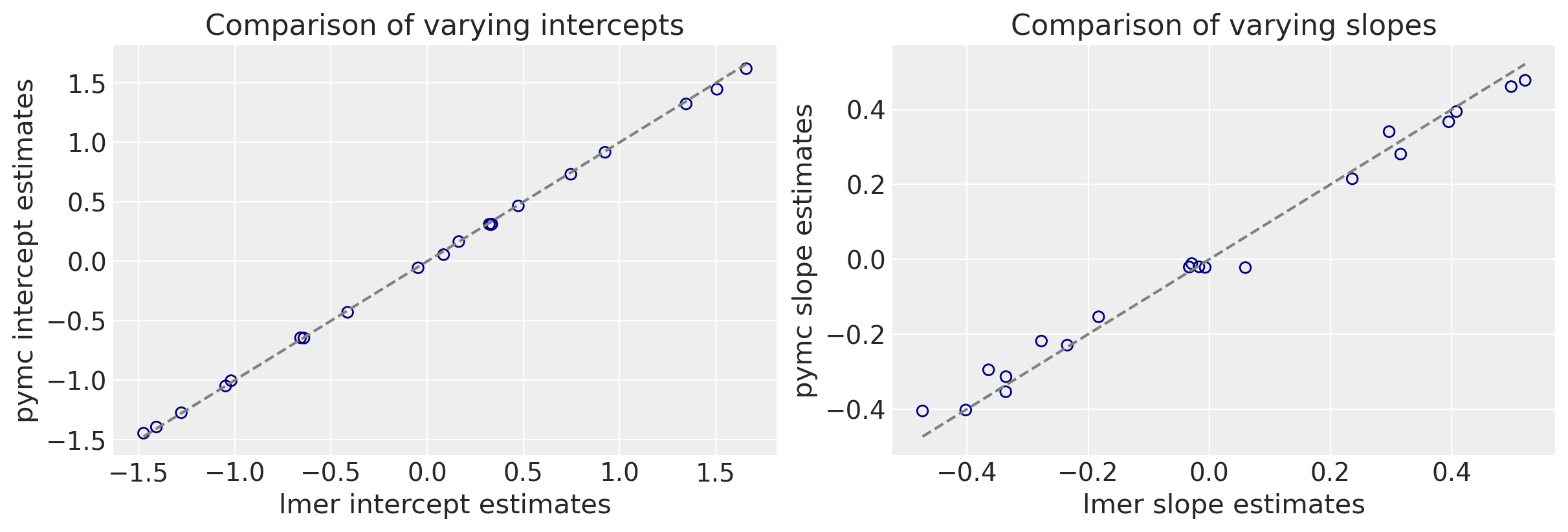
As you can see we get very similar intercepts and slopes for the cafe-specific estimates (varying effects) for the intercept and slope between the lmer and pymc approaches.

Summary

Here in this post, I set out to compare different mixed model approaches. I looked at the equations and the programmatic implementations. I concluded by showing how the two methods can arrive at the same answer. It required a careful understanding of the differences in equations and coding language- and package-specific implementations. There were various points of writing this post that confused me but it provided opportunities for deeper understanding.

Acknowledgements and references

Acknowledgements

• Special shoutout to Patrick Robotham (@probot) from the University of Bayes Discord channel for helping me work through many of my confusions.
• Eric J. Daza about some discussions about mixed effects modeling. It reminded me about improving my knowledge in this area.
• Members of the Glymour group at UCSF for checking some of my code.

References

• UCLA introduction to linear mixed models.
• Richard McElreath’s Statistical Rethinking for my introduction to Bayesian multilevel modeling and the Statistical Rethinking Chapter 14 repo.
• Andrzej Gałecki and Tomasz Burzykowski’s Linear Mixed-Effecsts Models Using R which references the lme4 package. Dr. McElreath referenced this package as a non-Bayesian alternative in his book.
• Andrew Gelman wrote about why he doesn’t like using “fixed and random effects” (in a blog and in a paper).
• TJ Mahr’s partial pooling blog post.

%load_ext watermark
%watermark -n -u -v -iv -w -p aesara,aeppl

The watermark extension is already loaded. To reload it, use:
  %reload_ext watermark
Last updated: Tue Sep 13 2022

Python implementation: CPython
Python version       : 3.10.6
IPython version      : 8.4.0

aesara: 2.8.2
aeppl : 0.0.35

pymc      : 4.1.7
xarray    : 2022.6.0
pandas    : 1.4.3
sys       : 3.10.6 | packaged by conda-forge | (main, Aug 22 2022, 20:43:44) [Clang 13.0.1 ]
arviz     : 0.12.1
matplotlib: 3.5.3
aesara    : 2.8.2
numpy     : 1.23.2

Watermark: 2.3.1

%%R
sessionInfo()

R version 4.1.3 (2022-03-10)
Platform: x86_64-apple-darwin13.4.0 (64-bit)
Running under: macOS Monterey 12.5.1

Matrix products: default
LAPACK: /Users/blacar/opt/anaconda3/envs/pymc_env2/lib/libopenblasp-r0.3.21.dylib

locale:
[1] C/UTF-8/C/C/C/C

attached base packages:
[1] tools     stats     graphics  grDevices utils     datasets  methods  
[8] base     

other attached packages:
 [1] merTools_0.5.2  arm_1.13-1      MASS_7.3-58.1   lme4_1.1-30    
 [5] Matrix_1.4-1    forcats_0.5.2   stringr_1.4.1   dplyr_1.0.9    
 [9] purrr_0.3.4     readr_2.1.2     tidyr_1.2.0     tibble_3.1.8   
[13] ggplot2_3.3.6   tidyverse_1.3.2

loaded via a namespace (and not attached):
 [1] httr_1.4.4          jsonlite_1.8.0      splines_4.1.3      
 [4] foreach_1.5.2       modelr_0.1.9        shiny_1.7.2        
 [7] assertthat_0.2.1    broom.mixed_0.2.9.4 googlesheets4_1.0.1
[10] cellranger_1.1.0    globals_0.16.1      pillar_1.8.1       
[13] backports_1.4.1     lattice_0.20-45     glue_1.6.2         
[16] digest_0.6.29       promises_1.2.0.1    rvest_1.0.3        
[19] minqa_1.2.4         colorspace_2.0-3    httpuv_1.6.5       
[22] htmltools_0.5.3     pkgconfig_2.0.3     broom_1.0.0        
[25] listenv_0.8.0       haven_2.5.1         xtable_1.8-4       
[28] mvtnorm_1.1-3       scales_1.2.1        later_1.3.0        
[31] tzdb_0.3.0          googledrive_2.0.0   farver_2.1.1       
[34] generics_0.1.3      ellipsis_0.3.2      withr_2.5.0        
[37] furrr_0.3.1         cli_3.3.0           mime_0.12          
[40] magrittr_2.0.3      crayon_1.5.1        readxl_1.4.1       
[43] fs_1.5.2            future_1.27.0       fansi_1.0.3        
[46] parallelly_1.32.1   nlme_3.1-159        xml2_1.3.3         
[49] hms_1.1.2           gargle_1.2.0        lifecycle_1.0.1    
[52] munsell_0.5.0       reprex_2.0.2        compiler_4.1.3     
[55] rlang_1.0.4         blme_1.0-5          grid_4.1.3         
[58] nloptr_2.0.3        iterators_1.0.14    labeling_0.4.2     
[61] boot_1.3-28         gtable_0.3.0        codetools_0.2-18   
[64] abind_1.4-5         DBI_1.1.3           R6_2.5.1           
[67] lubridate_1.8.0     fastmap_1.1.0       utf8_1.2.2         
[70] stringi_1.7.8       parallel_4.1.3      Rcpp_1.0.9         
[73] vctrs_0.4.1         dbplyr_2.2.1        tidyselect_1.1.2   
[76] coda_0.19-4