Generating a predictive distribution for the number of people attending your party
A few years ago, not long after I started writing on this blog, I wrote a piece called The probability of making your Friday night party. Well, the opportunity has presented itself for predicting the number of people attending our party. This question came up between my wife and I since we’re trying to plan party logistics.
You might be asking yourself, “Ben, why don’t you just request RSVPs and get a more definitive number?” There are several reasons for this:
- The number of people in attendance is not only a key factor in party planning, but a factor that both affects and is affected by logistics. If you build the party, they will come. Therefore, it would be helpful to get a probability distribution for the number of attendees even before sending an Evite or request RSVPs.
- Friends and family have increasingly busy schedules and sometimes RSVPs aren’t reliable. We know they’d love to attend but have other barriers with complicated dependencies. Think caregiving for older parents, kids, or pets; travel preferences; already reserved tickets to sporting events; hair salon appointments (hey sometimes they’re hard to get). Cancellations last minute are increasingly common.
- In a post-pandemic world, it’s more acceptable to be a no-show if you’re experiencing any health symptoms.
- I’m a geek and thought of the fun way this can be answered with probability and statistics!
Here are some interesting aspects of the problem.
- Estimating the total number of people means considering the variable probabilities of attending across individuals. A grandmother will very likely come (probability of 0.9) while a co-worker with young kids is more of a toss-up (probability of 0.5). That’s why an initial, naive approach for using the binomial distribution for the entire guest list would not be optimal, since constant probability is assumed across individuals. However, one can apply binomial distribution to a group of friends or a family.
- Determining the expected value is relatively easy. Understanding the uncertainty is harder.
This problem was addressed by a 1993 paper by Ken Butler and Michael Stephens called The Distribution of a Sum of Binomial Random Variables . However, we can re-derive some of the work through reasoning with just a few fundamental probability rules:
- Identifying the probabilities of jointly occurring events which are otherwise independent means multiplying the probabilities of the individual events (“and” statements)
- Determining the total probability of several events occurring means adding the probabilities of the individual events (“or” statements)
- The sum of the probabilities of all possible events must add to 1.
Let’s get started!
import itertools
import matplotlib.pyplot as plt
import numpy as np
import pandas as pd
import seaborn as sns
from scipy.stats import binom
from scipy.stats._distn_infrastructure import rv_discrete_frozen
Probability distributions for each group
Here is a visualization of the problem. We can have probability distributions for different groups on an invite list. For explanation purposes, let’s imagine that we’re considering inviting three groups: a set of grandparents, neighbors, and a busy co-worker with their family with probability of attending as 90%, 75% for neighbors, and 50%, respectively. These groups would have binomial distributions that look like this.
# create a dataframe that holds the number and probability for each group
df_data = pd.DataFrame(
    {
        "group": ["Grandparents", "Neighbors", "Co-worker's family"],
        "n": [2, 4, 5],
        "p": [0.9, 0.5, 0.2]
    }
)
df_data
| group | n | p | |
|---|---|---|---|
| 0 | Grandparents | 2 | 0.9 |
| 1 | Neighbors | 4 | 0.5 |
| 2 | Co-worker's family | 5 | 0.2 |
# Visualize the probability distribution for each grouop
fig, axes = plt.subplots(1, 3, figsize=(16, 4), sharey=True)
for (i, row), ax  in zip(df_data.iterrows(), axes.flat):
    rv = binom(row['n'], row['p'])
    x = np.arange(row['n']+1)
    ax.bar(x, rv.pmf(x))
    ax.set(
        title = row['group'],
        ylim = (0, 1),
        xticks = x,
        xlabel = "Number attending",
        ylabel = "Probability"
        )
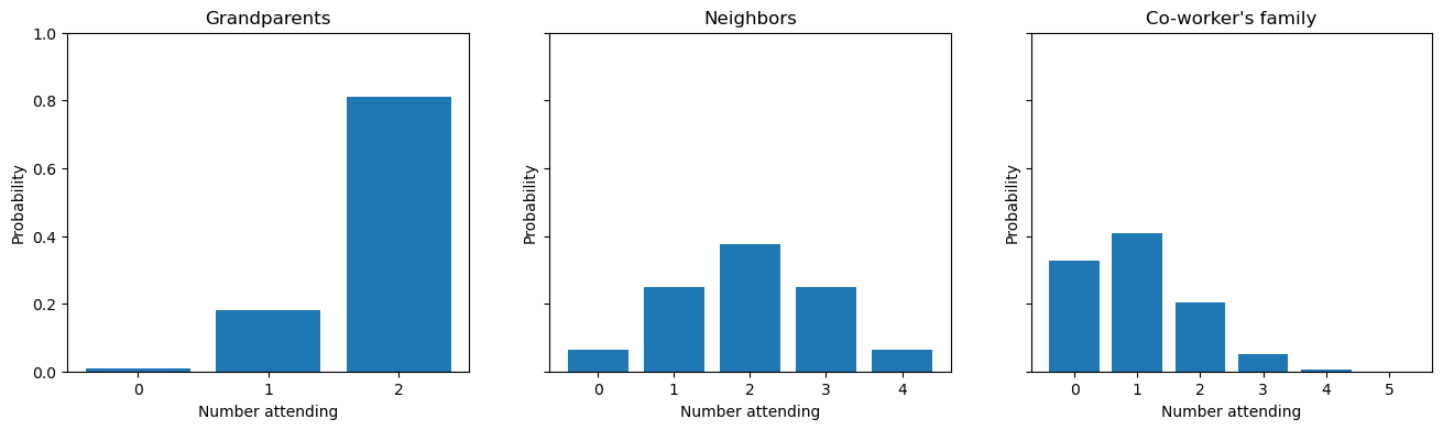
As you can see, it’s straighforward to get a distribution for each group. But how do we get a distribution for the total number of people attending?
Deriving the algorithm for the distribution of summed discrete random variables
We can look at the Butler and Stephens paper and see that they with both exact and approximate solutions. For our purposes, we’ll focus on the exact distribution, especially since there was this line from their paper: “With modern computing facilities, it is possible to calculate the exact distribution of S.” Remember this was written in 1993 when computers looked like this. Nevertheless, when you see the calculations carried out, you can appreciate why a statement was warranted and why they explored approximations, especially as the number of samples (possible attendees in this case) might scale.
The heart of the algorithm is the following equation.
\[P(Y + Z=j) = \sum_{i=0}^{j} P(Y=i) P(Z = j-i)\]$Y$ and $Z$ are two discrete random variables (e.g. integers) which makes sense since we don’t want a fraction of a person attending (unless it was Halloween). While they described $Y$ and $Z$ as variables with a binomial distribution, we can see later why this is not strictly necessary. Additionally, the equation only has $Y$ and $Z$ since they start with only two groups. Once that has been calculated the new distribution is the “new” $Y$ and the next group would be the “new” $Z$. This continues recursively until all groups have been accounted for.
We can derive the above formula with our putative invite example. We’ll go back to our dataframe where each row contains a group, the number of people ($n$), and the probability of attendance ($p$) but limit it to the first two rows where Grandparents is the $Y$ variable and Neighbors is the $Z$ variable.
df_data.head(2)
| group | n | p | |
|---|---|---|---|
| 0 | Grandparents | 2 | 0.9 |
| 1 | Neighbors | 4 | 0.5 |
And let’s look at each group’s probability distribution in table form.
# grandparents
i_vals_gp = range(df_data.loc[0, "n"] + 1)
Y = binom(df_data.loc[0, "n"], df_data.loc[0, "p"])
df_Y = pd.DataFrame({'x':i_vals_gp, 'probability':Y.pmf(i_vals_gp)})
df_Y
| x | probability | |
|---|---|---|
| 0 | 0 | 0.01 |
| 1 | 1 | 0.18 |
| 2 | 2 | 0.81 |
# neighbors
i_vals_nb = range(df_data.loc[1, "n"] + 1)
Z = binom(df_data.loc[1, "n"], df_data.loc[1, "p"])
df_Z = pd.DataFrame({'x':i_vals_nb, 'probability':Z.pmf(i_vals_nb)})
df_Z
| x | probability | |
|---|---|---|
| 0 | 0 | 0.0625 |
| 1 | 1 | 0.2500 |
| 2 | 2 | 0.3750 |
| 3 | 3 | 0.2500 |
| 4 | 4 | 0.0625 |
Now, we can consider the probabilities for each possibility of total attendance $j$. That means, $j$ is bounded by 0 (no one comes, wah wah) to 6 (everyone shows up). The probability for each value of $j$ can be deduced with probability rules. I’m italicizing some keywords below since we can link and statements to multiplication and or statements to addition.
- 0 total attendees ($j=0$): That means 0 grandparents show up and 0 neighbors show up. The probability of both happening means multiplying the probabilities ($0.01 \times 0.003906$).
- 1 total attendee ($j=1$): That means either 1 grandparent shows up and 0 neighbors show up ($0.18 \times 0.003906$) or 0 grandparents show up and 1 neighbor shows up ($0.01 \times 0.046875$). This means adding the two possibilities ($0.18 \times 0.003906 + 0.01 \times 0.046875$)
- 2 total attendees ($j=2$): Here’s where it starts get more complicated. That means either 2 grandparents show up and 0 neighbors show up ($0.81 \times 0.003906$) or 1 grandparent shows up and 1 neighbor shows up ($0.18 \times 0.046875$) or 0 grandparents show up and 2 neighbors show up ($0.01 \times 0.210938$). This means adding these three possibilities ($0.81 \times 0.003906 + 0.18 \times 0.046875 + 0.01 \times 0.210938$).
You can see the pattern and figure out the logic for the remaining values of $j$. Hopefully you can see now how this leads to the above equation. Let’s flesh this out with code.
def convert_binom_pmf(rv: rv_discrete_frozen) -> dict:
    """Convert a random variable's binomial distribution PMF to a dictionary.

    Parameters
    ----------
    rv
        Random variable Y representing discrete values

    Returns
    -------
    :
        Dictionary of probabilities for each j

    """
    j = rv.support()[1]
    return {x:rv.pmf(x) for x in range(j+1)}


def probability_for_j_total_people(
    j: int, rv_Y_prob: dict, rv_Z_prob: dict
) -> float:
    """Determine the probability of j people attending, given two random variables.

    Parameters
    ----------
    j
        The number of total attendees.
    rv_Y_prob
        Probability distribution of random variable Y as a dictionary
    rv_Z_prob
        Probability distribution of random variable Y as a dictionary

    Returns
    -------
    :
        Total probability of j
    """
    combinations = itertools.product(range(j + 1), repeat=2)
    total_j_combinations = [(y, z) for y, z in combinations if y + z == j]  # gives all y+z combinations that add up to j
    prob = 0
    x = range(j + 1)
    for combo in total_j_combinations:
        if (combo[0] in rv_Y_prob) and (combo[1] in rv_Z_prob):
            prob_combo = rv_Y_prob[combo[0]] * rv_Z_prob[combo[1]]
            prob += prob_combo
    return prob
total_prob = 0   # sanity check that the total probability adds up to 1
j_prob = dict()  # cache the probabilities in a dictionary
max_attendees = df_data.head(2)['n'].sum()
for j in range(max_attendees + 1):
    rv_Y_prob = convert_binom_pmf(Y)
    rv_Z_prob = convert_binom_pmf(Z)
    prob = probability_for_j_total_people(j, rv_Y_prob, rv_Z_prob)
    print(f"Probability for {j} total people: {prob:0.5f}")
    j_prob[j] = prob
    total_prob += prob

print(f"\nTotal probability after accounting for all cases: {total_prob:0.4f}")
Probability for 0 total people: 0.00062
Probability for 1 total people: 0.01375
Probability for 2 total people: 0.09938
Probability for 3 total people: 0.27250
Probability for 4 total people: 0.34937
Probability for 5 total people: 0.21375
Probability for 6 total people: 0.05063

Total probability after accounting for all cases: 1.0000
Awesome! It looks like we’ve successfully carried out the equation. But remember we’ve only done the first two groups. The next step is to add in the remaining group (co-worker's family) using the same process. But the probability distribution of our new $Y$ variable is what we just calculated, which is now stored in a dictionary j_prob. As I indicated above, there’s really no requirement that the distribution be binomial. It just has to be discrete.
# Let's recall the n and p of the remaining group
df_data.tail(1)
| group | n | p | |
|---|---|---|---|
| 2 | Co-worker's family | 5 | 0.2 |
We can carry out the same steps.
# coworkers
i_vals_cw = range(df_data.loc[2, "n"] + 1)
new_Z = binom(df_data.loc[2, "n"], df_data.loc[2, "p"])
rv_new_Z_prob = convert_binom_pmf(new_Z)  # put in dictionary form for our function
rv_new_Z_prob
{0: 0.3276799999999998,
 1: 0.4095999999999999,
 2: 0.20479999999999987,
 3: 0.051200000000000016,
 4: 0.0064,
 5: 0.0003200000000000001}
df_data
| group | n | p | |
|---|---|---|---|
| 0 | Grandparents | 2 | 0.9 |
| 1 | Neighbors | 4 | 0.5 |
| 2 | Co-worker's family | 5 | 0.2 |
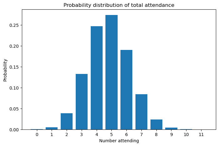
Recall that the putative total invite list was 11 people. Therefore, our probability distribution should give probabilities for each value between 0 and 11, inclusive.
j_prob_new = dict()  # cache the probabilities in a dictionary
for j in range(df_data["n"].sum() + 1):
    prob = probability_for_j_total_people(
        j, j_prob, rv_new_Z_prob
    )  # j_prob is what we calculated for the first two groups
    j_prob_new[j] = prob

f, ax = plt.subplots(figsize=(8, 5))

ax.bar(j_prob_new.keys(), j_prob_new.values())
ax.set(
    title="Probability distribution of total attendance",
    xticks=list(j_prob_new.keys()),
    xlabel="Number attending",
    ylabel="Probability",
);
A user-friendly function
OK! So it now looks like we have our final, exact distribution for the sum of all variables, what Butler and Stephens called $S$. We can make the production of this distribution much more user friendly with another couple of functions. Passing in our dataframe, we will produce a list of dictionaries, where each dictionary is a group’s probability distribution. Then this list will be passed into a second function to give our final answer. You can see at the assert statement that gives us the same answer that we derived above, step-by-step.
df_data
| group | n | p | |
|---|---|---|---|
| 0 | Grandparents | 2 | 0.9 |
| 1 | Neighbors | 4 | 0.5 |
| 2 | Co-worker's family | 5 | 0.2 |
def sum_of_discrete_rvs_exact_calculation(pmf_list: list) -> pd.Series:
    """Determine the probability distribution using recursion.

    Perform the exact calculation on the first two rows (e.g. random variables).
    If more than two rows exist, treat the resulting probability distribution as
    a random variable and add the third row. Repeat until all rows have been
    accounted for.

    Parameters
    ----------
    pmf_list
        A list of dictionaries containing the probability mass functions of
        different groups attending.

    Returns
    -------
    :
        Final probability distribution as a pandas Series
    """
    pmf_list = pmf_list.copy() # prevent the original list from being altered

    s_prob = dict()
    max_attendees = max(list(pmf_list[0].keys())) + max(list(pmf_list[1].keys()))
    for j in range(max_attendees + 1):
        prob = probability_for_j_total_people(
                j, pmf_list[0], pmf_list[1]
        )
        s_prob[j] = prob

    # base case
    if len(pmf_list) == 2:
        return s_prob

    # apply recursion
    else:
        # remove the first element and then replace the remaining first element with the new dictionary
        pmf_list.pop(0)
        pmf_list[0] = s_prob
        return sum_of_discrete_rvs_exact_calculation(pmf_list)
# put each group in a probability distribution
pmf_list_party = [convert_binom_pmf(binom(df_data.loc[i, "n"], df_data.loc[i, "p"])) for i in df_data.index]
assert j_prob_new == sum_of_discrete_rvs_exact_calculation(pmf_list_party)
%load_ext watermark
%watermark -n -u -v -iv -w
Last updated: Fri Apr 12 2024

Python implementation: CPython
Python version       : 3.11.7
IPython version      : 8.21.0

numpy     : 1.25.2
seaborn   : 0.13.2
matplotlib: 3.8.2
pandas    : 2.2.0

Watermark: 2.4.3