Escaping the Devil’s Funnel

Multi-level models are great for improving our estimates. However, the intuitive way these kinds of models are specified (which goes by the unhelpful name “centered” parameterization) can be notorious for producing posterior distributions that are difficult to sample using Markov chain Monte Carlo. This is because when a parameter (such as the scale variable of one distribution) depends on other parameters, the posterior can have weird shapes. This is the rationale for re-specifying the model into a “non-centered” parameterization.

One does not need a multi-level model to appreciate this concept. In the divergent transition section of Statistical Rethinking lecture 13 , Dr. McElreath illustrates the centered and non-centered parameterization ideas with what he calls “The Devil’s Funnel”. A funnel can be seen when plotting $\nu$ and x from the following centered paramaterization (figures shown below).

\[\nu \sim \text{Normal}(0, \sigma)\] \[x \sim \text{Normal}(0, \text{exp}(\nu))\]

This is numerically equivalent to the non-centered form. The noteworthy trick is setting $x$ from a stochastic relationship to a deterministic one and creating a new variable $z$ that is easier to sample.

\[\nu \sim \text{Normal}(0, \sigma)\] \[z \sim \text{Normal}(0, 1)\] \[x = z \times \text{exp}(\nu))\]

In an online discussion forum, we shared experiences with these kinds of parameterizations since it was around the same time lecture 13 of Statistical Rethinking was released. In the divergent transition section of the lecture, I noticed that the centered parameterization had a distribution that looked somewhat bivariate Gaussian when the value of $\sigma$ was low. I thought changing parameterizations wouldn’t affect sampling efficiency. I then asked at what value of $\sigma$ does the sampling efficiency matter. Let’s find out!

# boiler plate setup code
import arviz as az
import matplotlib.pyplot as plt
import numpy as np
import pandas as pd
import pymc3 as pm
import scipy.stats as stats
from scipy.special import expit
from scipy.special import logit
import seaborn as sns
import statsmodels.api as sm

%load_ext nb_black
%config InlineBackend.figure_format = 'retina'
%load_ext watermark
RANDOM_SEED = 8927
np.random.seed(RANDOM_SEED)
az.style.use("arviz-darkgrid")
az.rcParams["stats.hdi_prob"] = 0.89  # sets default credible interval used by arviz

def standardize(x):
    x = (x - np.mean(x)) / np.std(x)
    return x

The Devil’s Funnel variables were originally specified like this:

\[\nu \sim \text{Normal}(0, \sigma=3)\] \[x \sim \text{Normal}(0, \text{exp}(\nu))\]

The funnel gets more extreme with higher values for the standard deviation of $\nu$. Since there is no data here, this would be like manipulating priors only. I therefore experimented with different values for the standard deviation (sigma) of $\nu$.

# Generate a list of sigmas for the prior nu
sigmas = np.geomspace(0.025, 1, num=10)

# Create dictionaries for storage
# samples for plotting
traces_C = dict()
traces_NC = dict()

# summary results
summary_C = dict()
summary_NC = dict()

# number of divergences
div_C = dict()
div_NC = dict()

# Look at sigma values
sigmas

array([0.025     , 0.03766575, 0.05674836, 0.0854988 , 0.12881507,
       0.19407667, 0.29240177, 0.44054134, 0.66373288, 1.        ])

The following code evaluates each sigma value and uses that to build centered and non-centered models. I’ll save the results at the end of each model run and then plot the sampling metrics down below.

for sigma in sigmas:

    # Centered model
    with pm.Model() as mC:
        v = pm.Normal("v", 0.0, sigma)
        x = pm.Normal("x", 0.0, pm.math.exp(v))
        trace_mC = pm.sample(draws=1000, tune=1000, chains=4, return_inferencedata=False, progressbar=False)
        # Save results
        traces_C[sigma] = trace_mC
        summary_C[sigma] = az.summary(trace_mC)
        div_C[sigma] = trace_mC["diverging"].sum()

    # Non-centered model
    with pm.Model() as mNC:
        v = pm.Normal("v", 0.0, sigma)
        z = pm.Normal("z", 0.0, 1.0)
        # transformed variable
        x = pm.Deterministic("x", z*np.exp(v))
        trace_mNC = pm.sample(draws=1000, tune=1000, chains=4, return_inferencedata=False, progressbar=False)

        # Save results
        traces_NC[sigma] = trace_mNC
        summary_NC[sigma] = az.summary(trace_mNC)
        div_NC[sigma]= trace_mNC["diverging"].sum()

Auto-assigning NUTS sampler...
Initializing NUTS using jitter+adapt_diag...
Multiprocess sampling (4 chains in 4 jobs)
NUTS: [x, v]

(Removed the rest of the pymc output to save space. Notes about divergences are explored down below.)

Exploration of the joint distribution

We’ll plot the joint distribution of the centered-parameterization of $x$ and $\nu$ (blue) and see how that looks compared to the non-centered parameterization. In the latter, we’re sampling $z$ from a regular Gaussian distribution and getting $x$ through a deterministic transformation relationship.

sigmas_sampled = sigmas[1:len(sigmas):2]  # plot every other sigma evaluated

f, axes = plt.subplots(3, len(sigmas_sampled), figsize=(20, 8))

# top row: centered model
for sigma, ax in zip(sigmas_sampled, axes.flat[0:len(sigmas_sampled)]):
    samples_C = pm.trace_to_dataframe(traces_C[sigma])
    ax.scatter(samples_C['x'], samples_C['v'], alpha=0.2, facecolors='none', edgecolors='navy')

    sigma_str = '{:.3f}'.format(sigma)
    ax.set_title(f'sigma = {sigma_str}')
    ax.set_xlabel('x (stochastic)')
    if ax.is_first_col() & ax.is_first_row():
        ax.set_ylabel('centered\n\nv')

# middle row: non-centered model, z on x-axis
for sigma, ax in zip(sigmas_sampled, axes.flat[len(sigmas_sampled):2*len(sigmas_sampled)]):
    samples_NC = pm.trace_to_dataframe(traces_NC[sigma])
    ax.scatter(samples_NC['z'], samples_NC['v'], alpha=0.2, facecolors='none', edgecolors='darkgreen')

    ax.set_xlabel('z (stochastic)')
    if ax.is_first_col():
        ax.set_ylabel('non-centered\n\nv')

# bottom row: non-centered model, x on x-axis
for sigma, ax in zip(sigmas_sampled, axes.flat[2*len(sigmas_sampled):3*len(sigmas_sampled)]):
    samples_NC = pm.trace_to_dataframe(traces_NC[sigma])
    ax.scatter(samples_NC['x'], samples_NC['v'], alpha=0.2, facecolors='none', edgecolors='darkgreen')

    ax.set_xlabel('x (deterministic)')
    if ax.is_first_col() & ax.is_last_row():
        ax.set_ylabel('non-centered\n\nv')

plt.tight_layout()

<ipython-input-21-5993b7c4c1c1>:34: UserWarning: This figure was using constrained_layout==True, but that is incompatible with subplots_adjust and or tight_layout: setting constrained_layout==False. 
  plt.tight_layout()

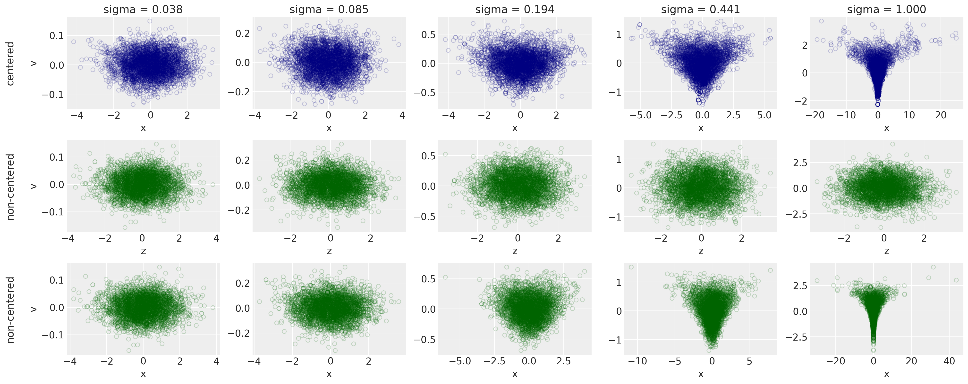
At the top is the centered target distribution with increasing values of $\sigma$. We can see that the Devil’s Funnel begins to form as $/sigma$ exceeds 0.2. However, the middle row looks like samples from a plain old bivariate Gaussian regression and doesn’t change. That’s because we’ve defined it to not change: it will always be $z \sim \text{Normal}(0,1)$ regardless of $\sigma$. The last row shows that we can get $x$ and our target distribution back with a deterministic transformation.

Let’s look at other metrics to inform us about sampling efficiency.

Number of divergences

f, ax1 = plt.subplots(figsize=(6, 4))
ax1.scatter(div_C.keys(), div_C.values(), color='navy')
ax1.plot(div_C.keys(), div_C.values(), color='navy', label='Centered')
ax1.scatter(div_NC.keys(), div_NC.values(), color='darkgreen')
ax1.plot(div_NC.keys(), div_NC.values(), color='darkgreen', label='Non-centered')
ax1.set(xlabel='sigma', ylabel='Number of divergences', title='Number of divergences\nCentered vs Non-centered')
ax1.legend()

<matplotlib.legend.Legend at 0x7fd419834520>

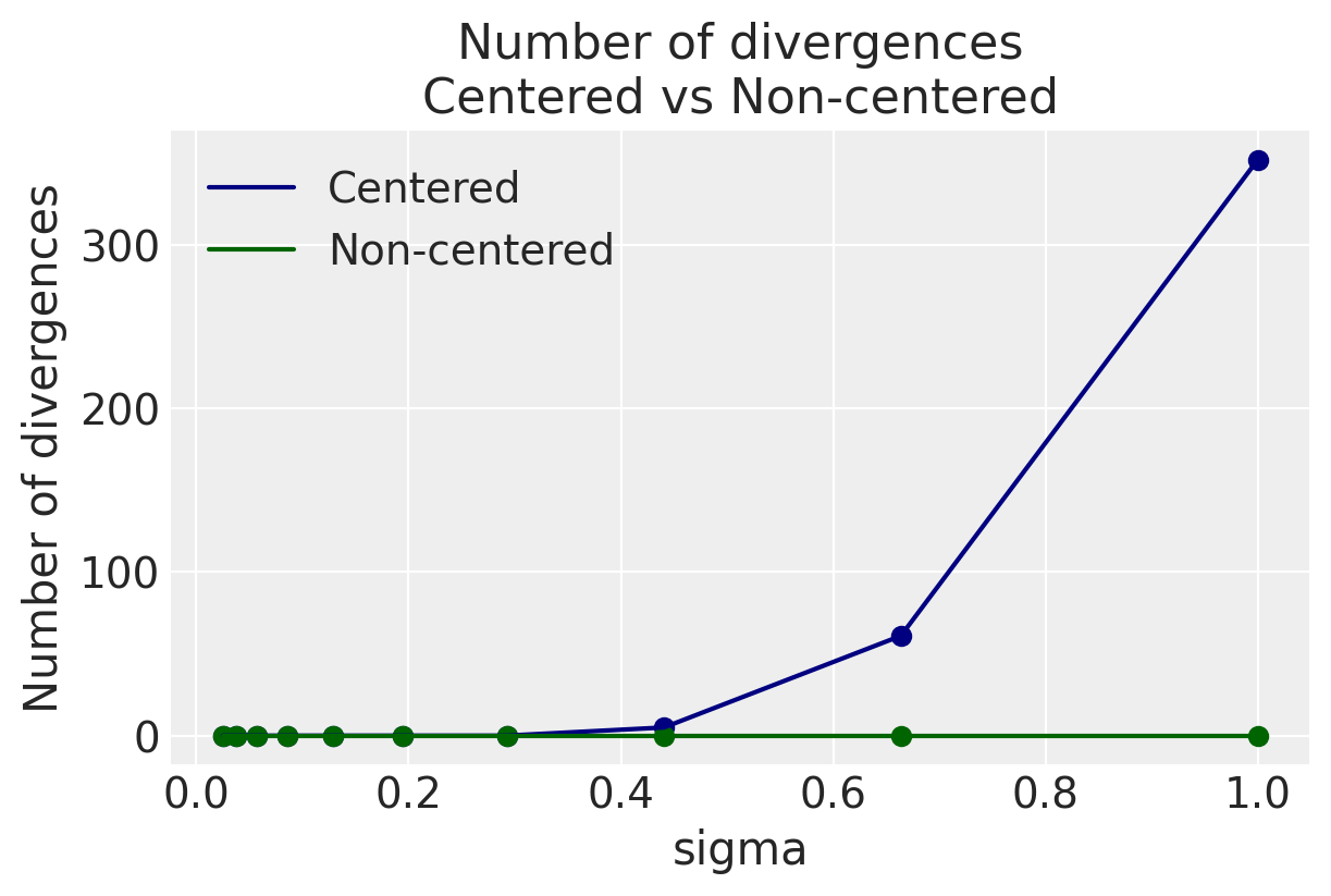
We don’t see any divergences at all in the non-centered paramaterization, regardless of $\sigma$. We can get away with the centered paramaterization only at low values of $\sigma$ as the bivariate plots suggest.

Number of effective samples and R-hat

# Put the summary results in one table to facilitate plotting
df_summary_C = pd.concat(pd.DataFrame(summary_C[sigma]).reset_index().rename(columns={'index': 'var'}) for sigma in sigmas).reset_index(drop=True)
df_summary_C['sigma'] = sorted(list(sigmas)*2)

df_summary_NC = pd.concat(pd.DataFrame(summary_NC[sigma]).reset_index().rename(columns={'index': 'var'}) for sigma in sigmas).reset_index(drop=True)
df_summary_NC['sigma'] = sorted(list(sigmas)*3)

f, ((ax1, ax2), (ax3, ax4)) = plt.subplots(2, 2, figsize=(12, 8))

# Top row (v) ---------

# plot centered ESS
df_centered_v = df_summary_C.loc[df_summary_C['var']=='v', :]
ax1.scatter(df_centered_v['sigma'], df_centered_v['ess_mean'], color='navy')
ax1.plot(df_centered_v['sigma'], df_centered_v['ess_mean'], color='navy', label='Centered')

ax2.scatter(df_centered_v['sigma'], df_centered_v['r_hat'], color='navy')
ax2.plot(df_centered_v['sigma'], df_centered_v['r_hat'], color='navy', label='Centered')

# plot non-centered ESS
df_noncentered_v = df_summary_NC.loc[df_summary_NC['var']=='v', :]
ax1.scatter(df_noncentered_v['sigma'], df_noncentered_v['ess_mean'], color='darkgreen')
ax1.plot(df_noncentered_v['sigma'], df_noncentered_v['ess_mean'], color='darkgreen', label='Non-centered')

ax2.scatter(df_noncentered_v['sigma'], df_noncentered_v['r_hat'], color='darkgreen')
ax2.plot(df_noncentered_v['sigma'], df_noncentered_v['r_hat'], color='darkgreen', label='Non-centered')

# plot decorations
ax1.legend()
ax1.set(xlabel='sigma', ylabel='ESS', xscale='linear', title='Effective sample size for v')

ax2.legend()
ax2.set(xlabel='sigma', ylabel='R-hat', xscale='linear', title='R-hat for v')

# Bottom row (x) ---------

# plot centered ESS
df_centered_x = df_summary_C.loc[df_summary_C['var']=='x', :]
ax3.scatter(df_centered_x['sigma'], df_centered_x['ess_mean'], color='navy')
ax3.plot(df_centered_x['sigma'], df_centered_x['ess_mean'], color='navy', label='Centered')

ax4.scatter(df_centered_x['sigma'], df_centered_x['r_hat'], color='navy')
ax4.plot(df_centered_x['sigma'], df_centered_x['r_hat'], color='navy', label='Centered')

# plot non-centered ESS
df_noncentered_x = df_summary_NC.loc[df_summary_NC['var']=='x', :]
ax3.scatter(df_noncentered_x['sigma'], df_noncentered_x['ess_mean'], color='darkgreen')
ax3.plot(df_noncentered_x['sigma'], df_noncentered_x['ess_mean'], color='darkgreen', label='Non-centered')

ax4.scatter(df_noncentered_x['sigma'], df_noncentered_x['r_hat'], color='darkgreen')
ax4.plot(df_noncentered_x['sigma'], df_noncentered_x['r_hat'], color='darkgreen', label='Non-centered')

# plot decorations
ax3.legend()
ax3.set(xlabel='sigma', ylabel='ESS', xscale='linear', title='Effective sample size for x')

ax4.legend()
ax4.set(xlabel='sigma', ylabel='R-hat', xscale='linear', title='R-hat for x')

f, ((ax1, ax2), (ax3, ax4)) = plt.subplots(2, 2, figsize=(12, 8))

# Top row (v) ---------

# plot centered ESS
df_centered_v = df_summary_C.loc[df_summary_C['var']=='v', :]
ax1.plot(df_centered_v['sigma'], df_centered_v['ess_mean'], marker='o', color='navy', label='Centered')
ax2.plot(df_centered_v['sigma'], df_centered_v['r_hat'], marker='o', color='navy', label='Centered')

# plot non-centered ESS
df_noncentered_v = df_summary_NC.loc[df_summary_NC['var']=='v', :]
ax1.plot(df_noncentered_v['sigma'], df_noncentered_v['ess_mean'], marker='o', color='darkgreen', label='Non-centered')
ax2.plot(df_noncentered_v['sigma'], df_noncentered_v['r_hat'], marker='o', color='darkgreen', label='Non-centered')

# plot decorations
ax1.legend()
ax1.set(xlabel='sigma', ylabel='ESS', xscale='linear', title='Effective sample size for v')
ax2.legend()
ax2.set(xlabel='sigma', ylabel='R-hat', xscale='linear', title='R-hat for v')

# Bottom row (x) ---------

# plot centered ESS
df_centered_x = df_summary_C.loc[df_summary_C['var']=='x', :]
ax3.plot(df_centered_x['sigma'], df_centered_x['ess_mean'], marker='o', color='navy', label='Centered')
ax4.plot(df_centered_x['sigma'], df_centered_x['r_hat'], marker='o', color='navy', label='Centered')

# plot non-centered ESS
df_noncentered_x = df_summary_NC.loc[df_summary_NC['var']=='x', :]
ax3.plot(df_noncentered_x['sigma'], df_noncentered_x['ess_mean'], marker='o', color='darkgreen', label='Non-centered')
ax4.plot(df_noncentered_x['sigma'], df_noncentered_x['r_hat'], marker='o', color='darkgreen', label='Non-centered')

# plot decorations
ax3.legend()
ax3.set(xlabel='sigma', ylabel='ESS', xscale='linear', title='Effective sample size for x')

ax4.legend()
ax4.set(xlabel='sigma', ylabel='R-hat', xscale='linear', title='R-hat for x')

[Text(0.5, 0, 'sigma'),
 Text(0, 0.5, 'R-hat'),
 None,
 Text(0.5, 1.0, 'R-hat for x')]

Conclusion

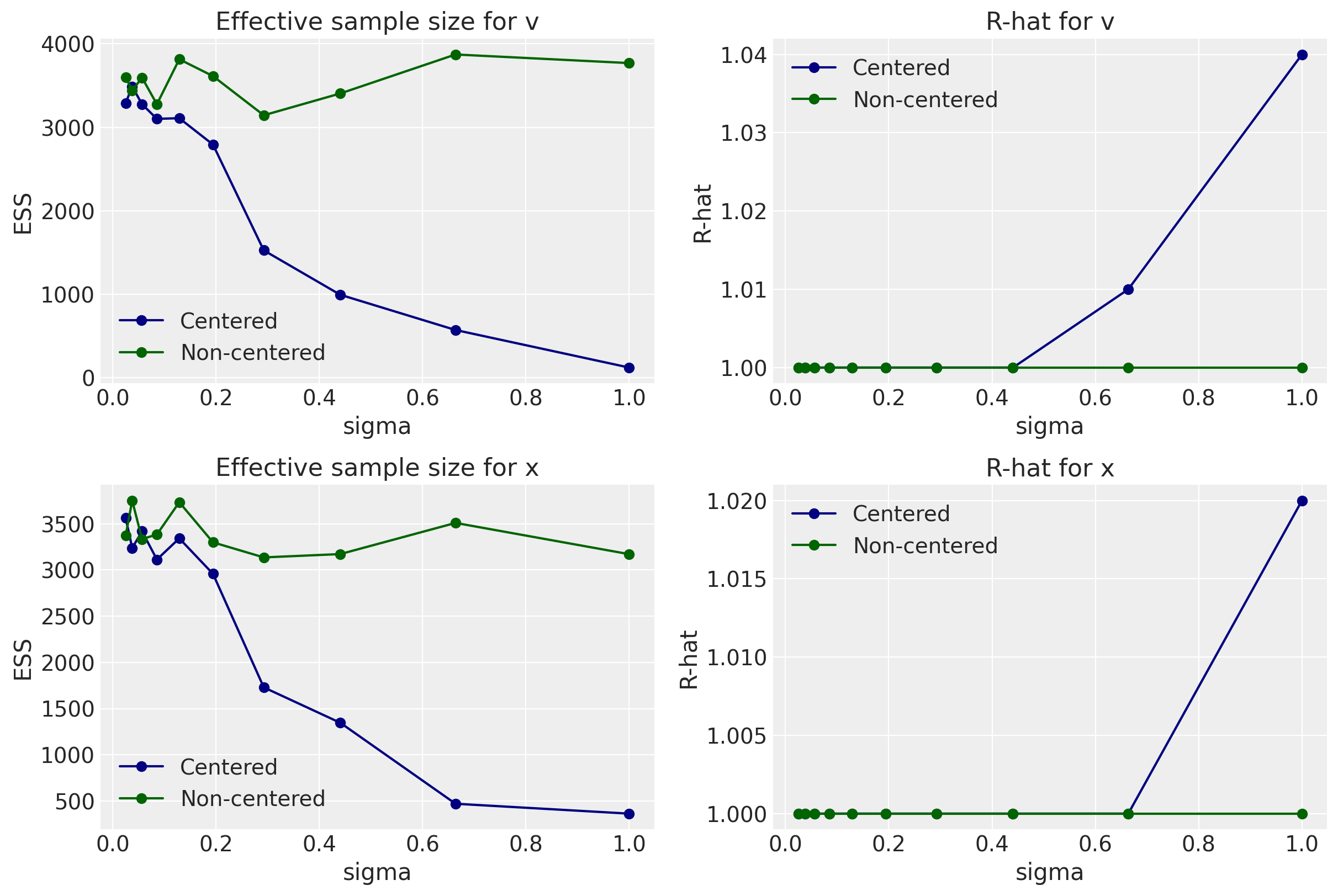
When looking at the number of divergences, effective sample size, and R-hat, smaller values of sigma result in good sampling whether it’s in the centered or non-centered form of the Devil’s Funnel equations. However, between 0.2 and 0.4, we begin to see indications that the non-centered form is clearly doing better.

Appendix: Environment and system parameters

%watermark -n -u -v -iv -w

Last updated: Sat Mar 26 2022

Python implementation: CPython
Python version       : 3.8.6
IPython version      : 7.20.0

pymc3      : 3.11.0
arviz      : 0.11.1
statsmodels: 0.12.2
numpy      : 1.20.1
sys        : 3.8.6 | packaged by conda-forge | (default, Jan 25 2021, 23:22:12) 
[Clang 11.0.1 ]
matplotlib : 3.3.4
pandas     : 1.2.1
scipy      : 1.6.0
seaborn    : 0.11.1

Watermark: 2.1.0