Sequences
This is the first in a series of posts about transformers, based on Andrej Karpathy’s amazing video Let’s build GPT: from scratch, in code, spelled out.
import torch
import seaborn as sns
from smart_open import open
sns.set_context("talk")
sns.set_palette("colorblind")
cb_palette = sns.color_palette()
The Shakespeare dataset
Why this as a teaching example? Common, open-source, intuitive for someone to understand
Real world dataset: The internet
# Inspect this link directly in the browser to see the data:
DATA_URL = "https://raw.githubusercontent.com/karpathy/char-rnn/master/data/tinyshakespeare/input.txt"
text = open(DATA_URL, "r").read()

# See the first 300 characters of the data:
print(text[0:300])
First Citizen:
Before we proceed any further, hear me speak.

All:
Speak, speak.

First Citizen:
You are all resolved rather to die than to famish?

All:
Resolved. resolved.

First Citizen:
First, you know Caius Marcius is chief enemy to the people.

All:
We know't, we know't.

First Citizen:
Let us
Character level tokenization
Why this as a teaching example? Simple, limited vocabulary
Real world: tokenizers like … yields very high vocabulary (xx number of tokens)
From this corpus, we’re able to derive a very simple vocabulary. Note that I’m showing the list of chars here so you can see special characters like newlines and spaces are part of the vocabulary.
chars = sorted(list(set(text)))
vocab_size = len(chars)


print(f"{vocab_size}\nunique characters: {chars}")
65
unique characters: ['\n', ' ', '!', '$', '&', "'", ',', '-', '.', '3', ':', ';', '?', 'A', 'B', 'C', 'D', 'E', 'F', 'G', 'H', 'I', 'J', 'K', 'L', 'M', 'N', 'O', 'P', 'Q', 'R', 'S', 'T', 'U', 'V', 'W', 'X', 'Y', 'Z', 'a', 'b', 'c', 'd', 'e', 'f', 'g', 'h', 'i', 'j', 'k', 'l', 'm', 'n', 'o', 'p', 'q', 'r', 's', 't', 'u', 'v', 'w', 'x', 'y', 'z']
Tensor setup
Why tensors? Why not strings, numpy matrices, etc.
stoi = {ch: i for i, ch in enumerate(chars)}
itos = {i: ch for i, ch in enumerate(chars)}


def encode(s):
    """Take a string, output a list of integers."""
    return [stoi[c] for c in s]


def decode(l):
    """Take a list of integers, output a string."""
    return "".join([itos[i] for i in l])


print(encode("hii there"))
print(decode(encode("hii there")))
[46, 47, 47, 1, 58, 46, 43, 56, 43]
hii there
Modern tokenizers include Google SentencePiece, OpenAI tiktoken.
Now tokenize the entire dataset. Why are we wrapping our tokens into a torch.tensor object? Practically, it plays nice with numpy or pandas, it can be moved to a GPU easily (x.to('cuda')), makes backpropagation calculation easy.
Note that specifying dtype=torch.long makes the data type integer. The pytorch default is float32 so constraining to integer is good practice to save memory.
data = torch.tensor(encode(text), dtype=torch.long)
print(data.shape, data.dtype)
print(data[:200])
torch.Size([1115394]) torch.int64
tensor([18, 47, 56, 57, 58,  1, 15, 47, 58, 47, 64, 43, 52, 10,  0, 14, 43, 44,
        53, 56, 43,  1, 61, 43,  1, 54, 56, 53, 41, 43, 43, 42,  1, 39, 52, 63,
         1, 44, 59, 56, 58, 46, 43, 56,  6,  1, 46, 43, 39, 56,  1, 51, 43,  1,
        57, 54, 43, 39, 49,  8,  0,  0, 13, 50, 50, 10,  0, 31, 54, 43, 39, 49,
         6,  1, 57, 54, 43, 39, 49,  8,  0,  0, 18, 47, 56, 57, 58,  1, 15, 47,
        58, 47, 64, 43, 52, 10,  0, 37, 53, 59,  1, 39, 56, 43,  1, 39, 50, 50,
         1, 56, 43, 57, 53, 50, 60, 43, 42,  1, 56, 39, 58, 46, 43, 56,  1, 58,
        53,  1, 42, 47, 43,  1, 58, 46, 39, 52,  1, 58, 53,  1, 44, 39, 51, 47,
        57, 46, 12,  0,  0, 13, 50, 50, 10,  0, 30, 43, 57, 53, 50, 60, 43, 42,
         8,  1, 56, 43, 57, 53, 50, 60, 43, 42,  8,  0,  0, 18, 47, 56, 57, 58,
         1, 15, 47, 58, 47, 64, 43, 52, 10,  0, 18, 47, 56, 57, 58,  6,  1, 63,
        53, 59])
# Look again how the data looks as integers, and then decode it back to characters to sanity check
print(" ".join(map(str, data.tolist()))[0:100])
print(" ".join(decode(data.tolist()))[0:100])
18 47 56 57 58 1 15 47 58 47 64 43 52 10 0 14 43 44 53 56 43 1 61 43 1 54 56 53 41 43 43 42 1 39 52
F i r s t   C i t i z e n :
 B e f o r e   w e   p r o c e e d   a n y   f u r t h e r ,   h e a r
Data splits
# Split data into train and validation tensor objects
n = int(0.9 * len(data))
train_data = data[:n]
val_data = data[n:]
Blocking and batching
Blocking (or context length)
It’s very computationally expensive to train the transformer by feeding it the whole text. Instead feed it chunks (or blocks) which is more computationally feasible.
In code, the maximum length of a chunk of data has to be specified. Here we’ll call it block_size but it might be referred to as context_length in other documentation.
block_size = 8

# We add a plus one so that we can have a target character for the last input character in the block
train_data[: block_size + 1]
tensor([18, 47, 56, 57, 58, 1, 15, 47, 58])
When we sample like this, it actually has multiple examples packed into it since every character follows each other. In this set of 9 tokens, there are 8 training examples. During training, each token in this block will have its own set of tokens behind it as a training example. In this way, there are at least two benefits: (1) the training will be more efficient and (2) the model will get used to seeing examples of different sizes.
x = train_data[:block_size]
y = train_data[1 : block_size + 1]
for t in range(block_size):
    context = x[: t + 1]
    target = y[t]
    print(f"When input is {context} target is: {target}")
When input is tensor([18]) target is: 47
When input is tensor([18, 47]) target is: 56
When input is tensor([18, 47, 56]) target is: 57
When input is tensor([18, 47, 56, 57]) target is: 58
When input is tensor([18, 47, 56, 57, 58]) target is: 1
When input is tensor([18, 47, 56, 57, 58,  1]) target is: 15
When input is tensor([18, 47, 56, 57, 58,  1, 15]) target is: 47
When input is tensor([18, 47, 56, 57, 58,  1, 15, 47]) target is: 58
What if your input size is longer than block size? In this simple architecture, you’d have to truncate the input.
Batching
Batching is stacking up multiple blocks of data into a tensor that is capable of being fed into a GPU if available. This is done for efficiency and to keep the GPUs busy since a lot of parallel processing can happen without the data talking or interacting with each other.
The code below is generalizing the above loop for a batch of data.
# torch.manual_seed(1337)
torch.manual_seed(9999)
batch_size = 4  # how many independent sequences will we process in parallel?
block_size = 8  # what is the maximum context length for predictions?


def get_batch(split):
    # generate a small batch of data of inputs x and targets y
    data = train_data if split == "train" else val_data
    # ix will return a tensor where values are randomly chosen between
    # 0 and len(data) - block_size and the
    # shape of the tensor will be (batch_size,)
    ix = torch.randint(len(data) - block_size, (batch_size,))

    # then it will get each block of training data
    x = torch.stack([data[i : i + block_size] for i in ix])
    y = torch.stack([data[i + 1 : i + block_size + 1] for i in ix])
    return x, y


xb, yb = get_batch("train")
print("inputs:")
print(xb.shape)
print(f"xb:\n {xb}")

print("targets:")
print(yb.shape)
print(f"yb:\n {yb}")
inputs:
torch.Size([4, 8])
xb:
 tensor([[ 1, 57, 47, 52, 57,  1, 51, 53],
        [43, 42, 43, 51, 54, 58, 47, 53],
        [53, 59,  1, 56, 59, 52,  1, 57],
        [56,  7, 57, 59, 47, 58, 43, 42]])
targets:
torch.Size([4, 8])
yb:
 tensor([[57, 47, 52, 57,  1, 51, 53, 57],
        [42, 43, 51, 54, 58, 47, 53, 52],
        [59,  1, 56, 59, 52,  1, 57, 53],
        [ 7, 57, 59, 47, 58, 43, 42,  1]])
len(train_data) - block_size
1003846
torch.randint(len(data) - block_size, (batch_size,))
tensor([162309, 283811, 193658, 667105])
for b in range(batch_size):  # batch dimension
    for t in range(block_size):  # time dimension
        context = xb[b, : t + 1]
        target = yb[b, t]

        print(f"When input is {context.tolist()} the target is: {target}")
When input is [1] the target is: 57
When input is [1, 57] the target is: 47
When input is [1, 57, 47] the target is: 52
When input is [1, 57, 47, 52] the target is: 57
When input is [1, 57, 47, 52, 57] the target is: 1
When input is [1, 57, 47, 52, 57, 1] the target is: 51
When input is [1, 57, 47, 52, 57, 1, 51] the target is: 53
When input is [1, 57, 47, 52, 57, 1, 51, 53] the target is: 57
When input is [43] the target is: 42
When input is [43, 42] the target is: 43
When input is [43, 42, 43] the target is: 51
When input is [43, 42, 43, 51] the target is: 54
When input is [43, 42, 43, 51, 54] the target is: 58
When input is [43, 42, 43, 51, 54, 58] the target is: 47
When input is [43, 42, 43, 51, 54, 58, 47] the target is: 53
When input is [43, 42, 43, 51, 54, 58, 47, 53] the target is: 52
When input is [53] the target is: 59
When input is [53, 59] the target is: 1
When input is [53, 59, 1] the target is: 56
When input is [53, 59, 1, 56] the target is: 59
When input is [53, 59, 1, 56, 59] the target is: 52
When input is [53, 59, 1, 56, 59, 52] the target is: 1
When input is [53, 59, 1, 56, 59, 52, 1] the target is: 57
When input is [53, 59, 1, 56, 59, 52, 1, 57] the target is: 53
When input is [56] the target is: 7
When input is [56, 7] the target is: 57
When input is [56, 7, 57] the target is: 59
When input is [56, 7, 57, 59] the target is: 47
When input is [56, 7, 57, 59, 47] the target is: 58
When input is [56, 7, 57, 59, 47, 58] the target is: 43
When input is [56, 7, 57, 59, 47, 58, 43] the target is: 42
When input is [56, 7, 57, 59, 47, 58, 43, 42] the target is: 1
Now feed these into a transformer.
Bigram Language Model (without the loss function)
See his video more details.
Why this as a teaching example? Literally use only current (one) character to predict the next (and only one) character.
Real world: tokenizers like … yields very high vocabulary (xx number of tokens)
Before going into the model, let’s explain some pytorch functions. Let’s start with nn.Embedding. We’ll initialize it with two parameters, each will be vocab_size. The first one represents the input, since we need a row for each input token. The second vocab_size represents the output, which is every possible next token. The values of the embedding table itself start off as random but then will be learned during back propagation.
In this post, we’ll focus on the very basics and stop before we introduce the loss function. The model with the loss function will be covered in a later post.
import torch
import torch.nn as nn
from torch.nn import functional as F

torch.manual_seed(1337)
<torch._C.Generator at 0xfffea0e51290>
What does nn.Embedding give us? Here, we’re inspecting the values. (The first set of random numbers set by the random seed are consumed here. It will change if you re-run the cell.)
# .detach removes gradient tracking, .cpu moves the tensor to CPU memory, .numpy converts into numpy array
nn.Embedding(vocab_size, vocab_size).weight.detach().cpu().numpy()
array([[ 0.18077157, -0.06998809, -0.3596235 , ...,  1.6097364 ,
        -0.40322772, -0.8344702 ],
       [ 0.5978008 , -0.05140588, -0.06455874, ..., -1.4649245 ,
        -2.0555017 ,  1.8274626 ],
       [ 1.3035277 , -0.450132  ,  1.3471215 , ...,  0.19098009,
        -0.34250784,  1.7955089 ],
       ...,
       [ 0.4221906 , -1.8110788 , -1.011825  , ...,  0.54622185,
         0.2787799 ,  0.7279968 ],
       [-0.8108565 ,  0.24097146, -0.11390407, ...,  1.4508699 ,
         0.18363355,  0.30638522],
       [-1.4322455 , -0.28099647, -2.2789013 , ..., -0.55506617,
         1.0665984 ,  0.5363513 ]], shape=(65, 65), dtype=float32)
class BigramLanguageModel(nn.Module):
    def __init__(self, vocab_size):
        super().__init__()
        self.token_embedding_table = nn.Embedding(vocab_size, vocab_size)

    def forward(self, idx, targets):
        # idx and targets are both (B, T) tensor of integers
        # targets not created yet but it will be used later to compute the loss function
        # for each idx, it is plucking out the idx-th row out of that embedding table
        # logits is shape (B,T,C)
        logits = self.token_embedding_table(idx)

        return logits
Let’s initialize the model to inspect the token embeddings resulting from our input and the output. We have to set the seed again to see the same random numbers as above.
# note I'm setting the seed here again to get the same random numbers as above
torch.manual_seed(1337)
m = BigramLanguageModel(vocab_size)  # initialize the model
Then we’ll pass in xb which we already defined above as our batch of training data. It will get processed through the forward function, which returns another embedding at each B and T.
out = m(xb, yb)  # pass in the input and targets to the model, but targets not used yet
print(out.shape)  # for each example (B) and time step (T), return an embedding (C)
torch.Size([4, 8, 65])
Let’s remind ourselves what is going on. We’re providing an input xb where each value represents a token.
xb
tensor([[ 1, 57, 47, 52, 57,  1, 51, 53],
        [43, 42, 43, 51, 54, 58, 47, 53],
        [53, 59,  1, 56, 59, 52,  1, 57],
        [56,  7, 57, 59, 47, 58, 43, 42]])
Let’s look at the first value of xb which is a 1. We simply look at the token embedding table at the 1 indexed row.
m.token_embedding_table.weight[1, :]
tensor([ 0.5978, -0.0514, -0.0646, -0.4970,  0.4658, -0.2573, -1.0673,  2.0089,
        -0.5370,  0.2228,  0.6971, -1.4267,  0.9059,  0.1446,  0.2280,  2.4900,
        -1.2237,  1.0107,  0.5560, -1.5935, -1.2706,  0.6903, -0.1961,  0.3449,
        -0.3419,  0.4759, -0.7663, -0.4190, -0.4370, -1.0012, -0.4094, -1.6669,
        -1.3651, -0.1655,  0.9623,  0.0315, -0.7419, -0.2978,  0.0172, -0.1772,
        -0.1334,  0.2940,  1.3850,  0.1209,  2.5418, -0.6405, -1.9740, -0.3296,
         0.0080,  0.9262, -1.8846,  0.1670,  0.4586, -1.7662,  0.5860,  1.7510,
         0.2807,  0.3110, -0.6538, -0.6576,  0.3184, -0.5496, -1.4649, -2.0555,
         1.8275], grad_fn=<SelectBackward0>)
m.token_embedding_table.weight
Parameter containing:
tensor([[ 0.1808, -0.0700, -0.3596,  ...,  1.6097, -0.4032, -0.8345],
        [ 0.5978, -0.0514, -0.0646,  ..., -1.4649, -2.0555,  1.8275],
        [ 1.3035, -0.4501,  1.3471,  ...,  0.1910, -0.3425,  1.7955],
        ...,
        [ 0.4222, -1.8111, -1.0118,  ...,  0.5462,  0.2788,  0.7280],
        [-0.8109,  0.2410, -0.1139,  ...,  1.4509,  0.1836,  0.3064],
        [-1.4322, -0.2810, -2.2789,  ..., -0.5551,  1.0666,  0.5364]],
       requires_grad=True)
See how to edit this: the output is the same as the input
Since the output of the BigramLanguageModel is just getting the embedding of the next character ($i + 1$), we would expect it to be the same values as the current character ($i) in the input at this point, before any training has happened. Let’s look at the first example
out
tensor([[[ 0.5978, -0.0514, -0.0646,  ..., -1.4649, -2.0555,  1.8275],
         [-0.5201,  0.2831,  1.0847,  ..., -0.0198,  0.7959,  1.6014],
         [ 1.6515, -0.0424, -0.7355,  ...,  0.8682,  2.0593, -0.8159],
         ...,
         [ 0.5978, -0.0514, -0.0646,  ..., -1.4649, -2.0555,  1.8275],
         [-1.4177,  0.8682, -0.9121,  ..., -0.6264,  1.2195,  0.2068],
         [-0.1324, -0.5489,  0.1024,  ..., -0.8599, -1.6050, -0.6985]],

        [[ 0.3323, -0.0872, -0.7470,  ..., -0.6716, -0.9572, -0.9594],
         [ 1.0726,  0.7295, -0.6665,  ...,  0.3115, -1.7675,  0.6818],
         [ 0.3323, -0.0872, -0.7470,  ..., -0.6716, -0.9572, -0.9594],
         ...,
         [ 0.2475, -0.6349, -1.2909,  ...,  1.3064, -0.2256, -1.8305],
         [ 1.6515, -0.0424, -0.7355,  ...,  0.8682,  2.0593, -0.8159],
         [-0.1324, -0.5489,  0.1024,  ..., -0.8599, -1.6050, -0.6985]],

        [[-0.1324, -0.5489,  0.1024,  ..., -0.8599, -1.6050, -0.6985],
         [-0.4002,  0.3302,  1.5454,  ...,  1.3688,  0.4620,  0.2040],
         [ 0.5978, -0.0514, -0.0646,  ..., -1.4649, -2.0555,  1.8275],
         ...,
         [-0.2103,  0.4481,  1.2381,  ...,  1.3597, -0.0821,  0.3909],
         [ 0.5978, -0.0514, -0.0646,  ..., -1.4649, -2.0555,  1.8275],
         [-0.5201,  0.2831,  1.0847,  ..., -0.0198,  0.7959,  1.6014]],

        [[-0.6722,  0.2322, -0.1632,  ...,  0.1390,  0.7560,  0.4296],
         [ 0.2410, -1.6206,  0.4488,  ..., -0.6825, -1.6026, -0.1336],
         [-0.5201,  0.2831,  1.0847,  ..., -0.0198,  0.7959,  1.6014],
         ...,
         [ 0.2475, -0.6349, -1.2909,  ...,  1.3064, -0.2256, -1.8305],
         [ 0.3323, -0.0872, -0.7470,  ..., -0.6716, -0.9572, -0.9594],
         [ 1.0726,  0.7295, -0.6665,  ...,  0.3115, -1.7675,  0.6818]]],
       grad_fn=<EmbeddingBackward0>)
out[0, 1, :]
tensor([-0.5201,  0.2831,  1.0847,  1.9905,  0.7763, -0.8460,  0.8437,  0.7905,
        -0.5287, -0.1187,  0.6618, -0.6682, -1.8731,  0.7459,  2.1471,  1.0535,
        -0.7480,  2.0704, -1.1879, -0.7858,  0.1276, -0.9183,  0.5782, -1.7134,
        -1.2302, -0.4149, -0.9652, -0.9685, -0.2536, -1.0255, -0.9492, -0.1503,
         0.4905, -1.1986,  1.0955, -0.5802,  0.0199, -2.0645, -0.0617, -0.4054,
        -0.7169,  0.9026, -0.3288, -0.2391, -1.0618, -0.1223, -1.4403,  0.8433,
        -0.7001,  0.9611,  0.8550,  0.4062, -2.2157, -0.3732, -0.6900,  0.4235,
         2.6768,  1.0813,  0.6548,  1.9577,  0.1433, -0.0627, -0.0198,  0.7959,
         1.6014], grad_fn=<SelectBackward0>)
out[0, 0, :] # first 0th example, first 0th time step, all vocab_size logits
tensor([ 0.5978, -0.0514, -0.0646, -0.4970,  0.4658, -0.2573, -1.0673,  2.0089,
        -0.5370,  0.2228,  0.6971, -1.4267,  0.9059,  0.1446,  0.2280,  2.4900,
        -1.2237,  1.0107,  0.5560, -1.5935, -1.2706,  0.6903, -0.1961,  0.3449,
        -0.3419,  0.4759, -0.7663, -0.4190, -0.4370, -1.0012, -0.4094, -1.6669,
        -1.3651, -0.1655,  0.9623,  0.0315, -0.7419, -0.2978,  0.0172, -0.1772,
        -0.1334,  0.2940,  1.3850,  0.1209,  2.5418, -0.6405, -1.9740, -0.3296,
         0.0080,  0.9262, -1.8846,  0.1670,  0.4586, -1.7662,  0.5860,  1.7510,
         0.2807,  0.3110, -0.6538, -0.6576,  0.3184, -0.5496, -1.4649, -2.0555,
         1.8275], grad_fn=<SelectBackward0>)
torch.all(m.token_embedding_table.weight[1] == out[0, 0, :])
tensor(True)
At the next time step for the first example of xb, the token represented by 57 has its own embedding and those values will appear in the out tensor of the following time step.
torch.all(m.token_embedding_table.weight[57] == out[0, 1, :])
tensor(True)
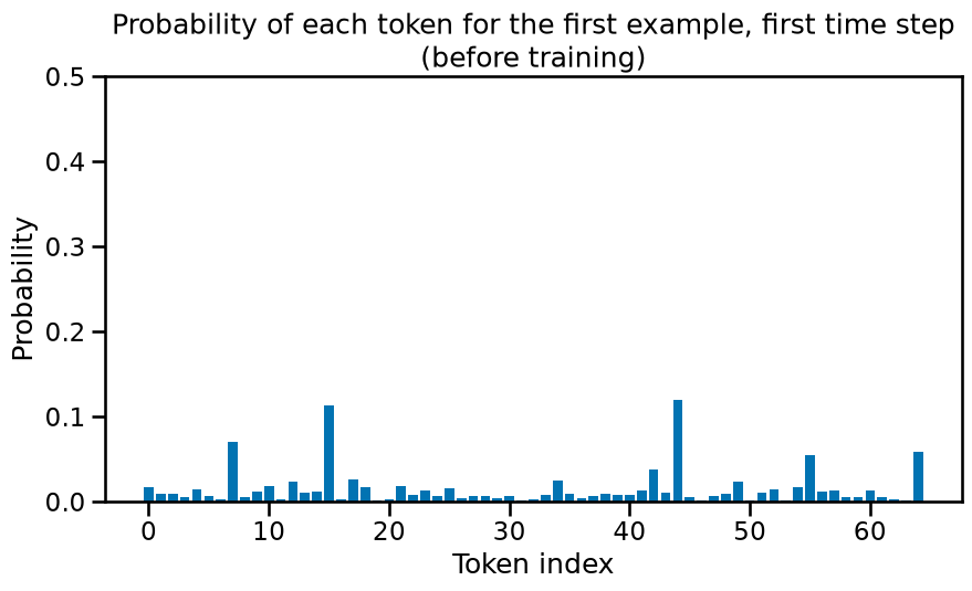
At this point, the probabilities of each token in the output are all relatively low which is what we’d expect since the model has had zero training. The probabilities at this point are just from random chance.
from scipy.special import softmax
from matplotlib import pyplot as plt


output_prob = softmax(out[0, 0, :].detach().cpu().numpy())
f, ax = plt.subplots(figsize=(10, 5))
ax.bar(x=range(len(output_prob)), height=output_prob)
ax.set(
    title="Probability of each token for the first example, first time step\n(before training)",
    ylim=(0, 0.5),
    xlabel="Token index",
    ylabel="Probability",
)
plt.show()
Let’s move towards that by introducing the loss function in later posts.
%load_ext watermark
%watermark -n -u -v -iv -w
Last updated: Fri, 28 Aug 2026

Python implementation: CPython
Python version       : 3.13.14
IPython version      : 9.14.1

matplotlib: 3.11.0
scipy     : 1.17.1
seaborn   : 0.13.2
smart_open: 7.6.1
torch     : 2.12.0

Watermark: 2.6.0